Control Valve Loop Tuning: Optimizing PID Control for Precision

In the intricate dance of industrial processes, precision is paramount. Whether it’s maintaining a specific temperature in a reactor, regulating pressure in a pipeline, or ensuring a consistent flow rate for a critical ingredient, the ability to maintain a process variable at its desired setpoint is the bedrock of efficiency, safety, and product quality. At the heart of this control lies a dynamic duo: the control valve and the PID controller. While the valve is the muscle, physically manipulating the process, the PID controller is the brain, making the decisions. However, a brilliant brain and a strong muscle are ineffective without a well-coordinated nervous system. This is where control valve loop tuning comes in – the art and science of harmonizing the controller’s actions with the characteristics of the valve and the process it governs.

A poorly tuned control loop is a silent saboteur. It can lead to oscillations that wreak havoc on equipment, increase energy consumption, produce off-spec products, and even create safety hazards. Conversely, a finely tuned loop is a masterpiece of engineering, responding swiftly and smoothly to disturbances, minimizing variability, and ultimately, boosting the bottom line. This comprehensive guide will delve into the intricacies of control valve loop tuning, exploring the fundamental principles of PID control, the nuances of control valve behavior, and a range of tuning methodologies designed to achieve precision.

The Anatomy of a Control Loop: A Symphony of Components

Before we dive into the tuning process, it’s essential to understand the key players in a typical control loop:

The Sensor: This is the lookout, responsible for measuring the process variable (PV) – be it temperature, pressure, flow, or level. The accuracy and responsiveness of the sensor are critical for effective control.
The Controller: The decision-maker, which is most commonly a Proportional-Integral-Derivative (PID) controller. It continuously compares the process variable from the sensor to the desired setpoint (SP) and calculates an output signal to the final control element.
The Final Control Element: This is the workhorse of the loop, the component that directly influences the process. In a vast number of industrial applications, this is a control valve. The controller’s output signal manipulates the position of the control valve, thereby adjusting the flow of a fluid or gas to influence the process variable.

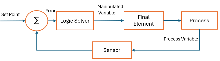
The seamless interaction of these three components is what constitutes a closed-loop control system. The goal of tuning is to optimize the controller’s response to ensure this interaction is as efficient and stable as possible.

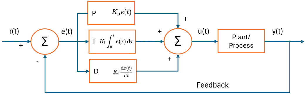
Decoding the PID Controller: The Three Pillars of Control

The magic of the PID controller lies in its three distinct modes of action, each playing a unique role in bringing the process variable to the setpoint.

Proportional (P) Action: The proportional term, governed by the controller gain ( $K_{c}$ ), provides an output that is directly proportional to the current error (the difference between the setpoint and the process variable). A higher gain results in a more aggressive response to errors. However, an excessively high gain can lead to instability and oscillations. Proportional control alone often results in a steady-state error, known as offset, where the process variable never quite reaches the setpoint.
Integral (I) Action: The integral term, characterized by the integral time or reset time ( $T_{i}$ ), is the memory of the controller. It continuously sums the error over time and adjusts the output to eliminate the offset left by the proportional action. A shorter integral time leads to a faster elimination of the offset, but it can also increase the risk of oscillations. The integral action is crucial for achieving precise setpoint tracking.
Derivative (D) Action: The derivative term, defined by the derivative time ( $T_{d}$ ), is the predictive element of the controller. It looks at the rate of change of the error and provides an output that dampens the response, preventing overshoot and oscillations. It essentially anticipates where the process variable is heading and takes corrective action beforehand. While derivative action can significantly improve loop stability, it is highly sensitive to measurement noise and is often used sparingly, particularly in noisy processes.

The Control Valve’s Personality: More Than Just a Valve

The control valve is not a perfect, instantaneous actuator. It has its own set of characteristics and limitations that must be considered during the tuning process.

Inherent Flow Characteristic: This describes the relationship between the valve’s travel (how much it’s open) and the flow rate under constant pressure conditions. The two most common characteristics are:
- Linear: The flow rate is directly proportional to the valve travel. These are often used in liquid level control and other processes where the pressure drop across the valve is relatively constant.
- Equal Percentage: Each increment of valve travel produces an equal percentage change in the existing flow. This type of valve is well-suited for processes with significant pressure drop variations and is commonly used in temperature and pressure control loops.
Installed Flow Characteristic: This is the actual relationship between valve travel and flow rate in a specific system, taking into account the dynamics of the entire process, including pumps and piping. The goal is to select a valve with an inherent characteristic that results in a relatively linear installed characteristic for easier tuning.

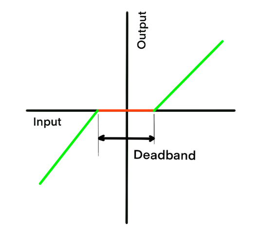
Valve Imperfections: Real-world control valves are subject to several non-ideal behaviors that can complicate tuning:
- Stiction (Static Friction): This is the force that must be overcome to initiate valve movement. It causes the valve to stick in one position until a significant change in the controller output forces it to move, often resulting in a sudden, large jump. Stiction is a major cause of control loop oscillations.
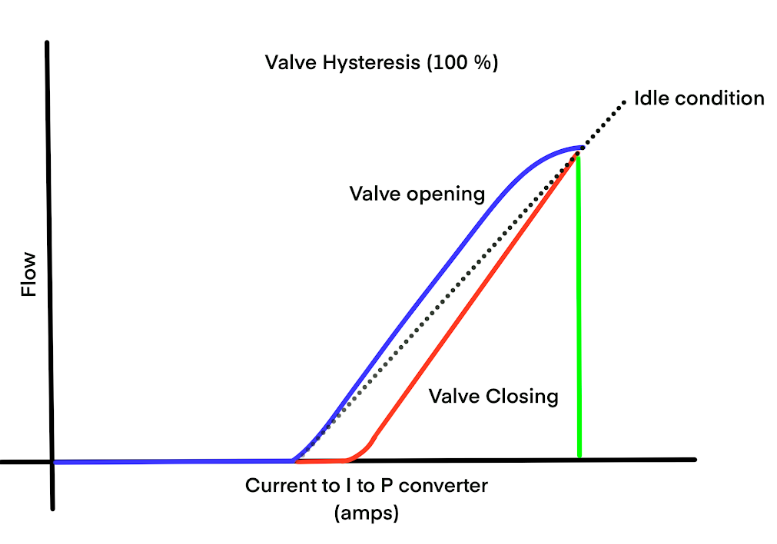
- Hysteresis: This is the difference in valve position for the same controller output signal, depending on whether the valve is opening or closing. It introduces a dead zone where a change in controller output results in no change in valve position.
- Deadband: This is the range through which the controller output can change without initiating any valve movement. It is often a combination of stiction and hysteresis.

The Art and Science of Tuning: Methodologies for Precision

With a solid understanding of the PID controller and the control valve, we can now explore the various methods for tuning the control loop.

1. Manual Tuning: The Intuitive Approach

This is the most basic method and relies heavily on the experience and intuition of the operator or engineer. The general process involves:

Setting the integral and derivative terms to their least active settings (maximum integral time, zero derivative time).
Gradually increasing the proportional gain until the loop begins to oscillate at a steady amplitude.
Reducing the gain by a factor of two.
Decreasing the integral time until any offset is corrected in a reasonable time.
If necessary, cautiously adding derivative action to improve response and reduce overshoot.

While this method can be effective for simple, non-critical loops, it is time-consuming, subjective, and can be risky for sensitive processes.

2. The Ziegler-Nichols Methods: A Classic Approach

Developed in the 1940s, the Ziegler-Nichols methods were among the first systematic approaches to PID tuning. They are known for producing aggressive, sometimes oscillatory, responses but provide an excellent starting point.

Closed-Loop (Ultimate Sensitivity) Method:
1. Follow the first two steps of manual tuning: set the controller to P-only mode and increase the gain until sustained oscillations occur.
2. Record the gain at which this happens as the ultimate gain ( $K_{u}$ ).
3. Measure the period of the oscillations as the ultimate period ( $P_{u}$ ).
4. Use the Ziegler-Nichols tuning table to calculate the P, I, and D parameters based on $K_{u}$ and $P_{u}$ .

Controller Type	$K_{c}$	$T_{i}$	$T_{d}$
P	$0.5 K_{u}$	–	–
PI	$0.45 K_{u}$	$P_{u} /1.2$	–
PID	$0.6 K_{u}$	$P_{u} /2$	$P_{u} /8$

Open-Loop (Process Reaction Curve) Method:
1. With the controller in manual mode, make a small, step change in the controller output.
2. Record the process variable’s response over time. This will typically resemble an “S” shape.
3. From the resulting graph, determine the process gain, dead time, and time constant.
4. Use a different set of Ziegler-Nichols formulas to calculate the tuning parameters.

While historically significant, the Ziegler-Nichols methods often require further fine-tuning to achieve a less aggressive response.

3. The Cohen-Coon Method: A Refinement for Self-Regulating Processes

The Cohen-Coon method is another open-loop technique that is particularly well-suited for processes with significant dead time. It often provides a more accurate model of the process than the Ziegler-Nichols method, leading to better initial tuning parameters. The procedure is similar to the Ziegler-Nichols open-loop method, involving a step test and analysis of the process reaction curve, but it uses more complex formulas to calculate the controller settings.

4. The Lambda Tuning Method: Designing for a Desired Response

The Lambda tuning method represents a more modern and sophisticated approach. Instead of aiming for a specific type of response (like the quarter-amplitude damping of Ziegler-Nichols), Lambda tuning allows the engineer to specify the desired closed-loop response time, known as Lambda ( $λ$ ).

A larger Lambda value results in a slower, more robust response, while a smaller Lambda value yields a faster, more aggressive response. This method is particularly advantageous because it:

Decouples Setpoint Tracking and Disturbance Rejection: It allows for separate tuning for how the loop responds to changes in the setpoint versus how it handles external disturbances.
Provides Robustness: Lambda-tuned loops are generally more tolerant of changes in process dynamics.
Is Highly Intuitive: The single Lambda parameter directly relates to the desired performance of the loop.

The Lambda tuning method also relies on a process model obtained from a step test, similar to the open-loop methods mentioned above.

Practical Considerations for Real-World Tuning

Beyond the theoretical methodologies, successful control loop tuning requires a pragmatic, hands-on approach.

Know Your Process: Before you touch any tuning parameters, have a thorough understanding of the process dynamics. Is it fast or slow? Does it have significant dead time? What are the potential sources of disturbances?
Address Mechanical Issues First: No amount of clever tuning can compensate for a faulty control valve. Before tuning, check for and address issues like stiction, hysteresis, and incorrect valve sizing.
Use Appropriate Tools: Modern process control systems and dedicated software offer powerful tools for loop tuning. These can automate step tests, calculate tuning parameters using various methods, and simulate the response before implementing it on the live process.
Tune in the Appropriate Controller Mode: The tuning should be performed in the controller mode that will be used during normal operation (e.g., automatic mode).
Make Small, Incremental Changes: Especially on critical loops, avoid making large, sudden changes to the tuning parameters.
Document Everything: Keep detailed records of all tuning changes, including the initial and final parameters, the tuning method used, and the observed response. This information is invaluable for future troubleshooting and optimization.
Test and Validate: After tuning, test the loop’s response to both setpoint changes and induced disturbances to ensure it performs as expected under various conditions.

The Payoff: The Tangible Benefits of Precision Control

Investing the time and effort to properly tune control valve loops yields significant returns:

Improved Product Quality: Consistent process control leads to a more uniform product, reducing waste and rework.
Increased Efficiency: Stable operation at the optimal setpoint can lead to reduced energy consumption and raw material usage.
Enhanced Safety: A well-tuned loop is a predictable loop. This reduces the risk of dangerous process excursions that could lead to equipment damage or personnel injury.
Extended Equipment Life: Smooth, stable control minimizes the wear and tear on control valves, pumps, and other process equipment.
Increased Throughput: By minimizing oscillations and off-spec product, overall production rates can often be increased.

Conclusion: A Continuous Journey of Optimization

Control valve loop tuning is not a one-time event. It is a continuous process of monitoring, analyzing, and optimizing. As processes change, equipment wears, and production demands evolve, the tuning parameters that were once optimal may need to be revisited.

By combining a solid theoretical understanding of PID control with a practical awareness of control valve behavior and a systematic approach to tuning, engineers and technicians can transform their control loops from sources of frustration into paragons of precision. In the competitive landscape of modern industry, the pursuit of optimized control is no longer a luxury – it is a necessity for achieving operational excellence. The finely tuned control loop, working silently and efficiently in the background, is a testament to the power of engineering to bring order and precision to a complex world.