
Instrumentation and Control Engineering (ICE) – Complete Over view
Part I: Foundations of Instrumentation and Control
Section 1: An Introduction to Process Control
The modern industrial landscape, from sprawling chemical plants to high-precision pharmaceutical laboratories, is built upon a foundation of automation. This automation is not merely a matter of machinery; it is an intricate interplay of measurement, analysis, and action, governed by the principles of instrumentation and control. This field represents the technological nervous system of industrial complexes, enabling processes to achieve levels of efficiency, safety, and quality that would be unattainable through manual operation alone.1 To comprehend the sophisticated systems that manage these operations, one must first understand the distinct yet deeply intertwined disciplines that form their basis: instrumentation and control engineering.
1.1 Defining Instrumentation: The Science of Measurement
At its core, instrumentation is the science and technology of measurement. It is the discipline concerned with the design, construction, and maintenance of devices that detect and quantify the physical and chemical characteristics of a process. These characteristics, known as process variables (PVs), encompass a vast range of parameters critical to industrial operations, including pressure, temperature, flow rate, liquid level, pH, humidity, force, and rotational speed.
The function of instrumentation is to provide the raw, empirical data that serves as the sensory input for any control strategy. It is the means by which a system gains awareness of its own state and the state of its environment. Without accurate, reliable, and timely measurement, any subsequent attempt at control is fundamentally flawed—an action taken without knowledge. Therefore, instrumentation is the essential prerequisite for control, forming the first link in the chain of automated process management. The quality, quantity, and overall efficiency of an industrial output are directly related to the quality of its instrumentation and control systems. Click to view the video for Instrumentation and control Engineering. (ICE) overview
1.2 Defining Instrumentation and Control Engineering : The Application of Control Theory
If instrumentation provides the senses, control engineering provides the intelligence and the capacity for action. Control engineering, also known as control systems engineering, is the discipline that applies control theory to design systems that exhibit desired behaviors, often with minimal or no human intervention. This field leverages mathematical modeling to understand the dynamics of a process and to create algorithms and logic that can manipulate system inputs to achieve a specific outcome.
The primary objective of a control engineer is to take the stream of data provided by instrumentation and use it to make corrective adjustments. These systems employ sensors to measure the output variable of a device and provide feedback to a controller, which then makes corrections to guide the system’s performance toward a desired target. Applications range from the familiar cruise control system in an automobile, which automatically regulates speed, to the highly complex, multi-variable control schemes that manage entire manufacturing facilities and process plants. The essence of control engineering is the transformation of measurement into purposeful manipulation.
1.3 The Synthesis: Instrumentation and Control Engineering (I&C) as a Discipline
Instrumentation and Control (I&C) Engineering is the synergistic integration of these two foundational fields. It is a multi-disciplinary branch of engineering that encompasses the complete lifecycle of systems that measure and control process variables, from initial conception and design to implementation, maintenance, and management. I&C engineers are tasked with designing, developing, testing, installing, and maintaining the equipment that automates the monitoring and control of machinery and processes. Click here to see complete control system blogs
This discipline is inherently holistic, drawing heavily upon principles from electrical, mechanical, chemical, and computer engineering to create robust and effective automation solutions. The role of the I&C engineer is to ensure that these integrated systems operate efficiently, effectively, and safely, forming the backbone of modern industrial automation.
The relationship between the instrumentation and control functions within this discipline is one of absolute dependency, but it can also be a source of significant operational challenges. Instrumentation provides the awareness of the process state, while control provides the action to modify that state. A failure in the measurement domain can easily be misdiagnosed as a failure in the control domain, and vice versa. Anecdotal evidence from the field reveals a common dynamic where an instrument engineer might attribute a fault to a “code problem,” while a controls engineer might blame a faulty sensor. This points to a deeper organizational reality: the most effective I&C systems are managed not by siloed teams, but by integrated groups that approach diagnostics with a systems-thinking perspective. They recognize that a drifting sensor can manifest as what appears to be a poorly tuned controller, and an erratic control signal can make a perfectly functional instrument seem faulty. The success of an I&C system is therefore not purely a technical achievement but also a reflection of an organization’s ability to manage the integrated nature of the system itself.
1.4 Core Objectives: The “Why” of Instrumentation and Control Engineering (ICE)
The implementation of instrumentation and control systems is not a purely technical endeavor; it is driven by fundamental business and operational imperatives that are directly linked to the profitability, safety, and long-term viability of an industrial enterprise.1 The overarching goals of an I&C engineer’s work are to maximize a set of key performance indicators.
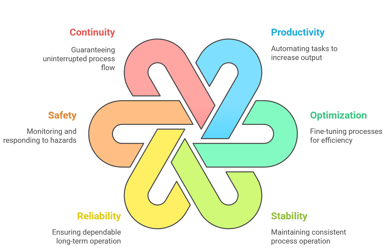
The primary objectives are to maximize:
- Productivity: Automating tasks and optimizing processes to increase throughput and output.
- Optimization: Fine-tuning process variables to achieve the most efficient use of raw materials and energy.
- Stability: Maintaining consistent and predictable process operation, reducing variability in product quality.
- Reliability: Ensuring the system operates dependably over long periods, minimizing unplanned downtime.
- Safety: Monitoring for hazardous conditions and implementing automated responses to protect personnel, equipment, and the environment.
- Continuity: Guaranteeing that processes can run continuously without interruption, which is critical in many industries.
These objectives often have critical, life-or-death implications. For instance, in a petrochemical plant, a temperature monitoring and control system is not merely an tool for optimizing a reaction; it is a vital safety system designed to prevent temperatures from reaching critical levels that could trigger a catastrophic explosion. This dual role of I&C—simultaneously enhancing performance and mitigating risk—underscores its central importance in modern industry.
Section 2: The Anatomy of the Control Loop
The fundamental building block of any automated industrial control system is the control loop. In a complex facility like a power plant or refinery, there may be hundreds or even thousands of individual control loops operating concurrently, each dedicated to regulating a specific aspect of the process. Understanding the architecture and components of a single control loop is essential to comprehending the function of these larger, more intricate systems.
2.1 The Process, Process Variable (PV), and Setpoint (SP)
Before examining the hardware, it is necessary to define the core concepts of the loop:
- The Process: This refers to the physical system or piece of equipment that is being controlled. It can be anything from a simple tank, a furnace, a chemical reactor, or a motor to an entire plant unit.
- The Process Variable (PV): This is the specific, measurable characteristic of the process that the control loop is designed to regulate. Examples include the temperature of a liquid, the pressure inside a vessel, the flow rate in a pipe, or the speed of a motor.
- The Setpoint (SP): This is the desired or target value for the process variable. It is the value at which the control system aims to maintain the PV.
- The Error: The driving force for any control action is the error, which is calculated as the difference between the setpoint and the current process variable (Error=SP−PV). The fundamental purpose of the control loop is to continuously work to minimize this error, driving it as close to zero as possible.
2.2 Core Components and Signal Flow
A typical industrial control loop consists of a series of interconnected components that form a continuous cycle of measurement, comparison, computation, and action. The flow of information and control signals through these components defines the operation of the loop.
2.2.1 Sensors and Primary Elements: The System’s Senses
The control loop’s interaction with the physical world begins with the Primary Element, or Sensor. This device is in direct contact with the process and is responsible for measuring the process variable.11 It acts as the “eyes of the control system,” providing the initial raw measurement.
A sensor works by converting a physical property, such as heat, force, or fluid velocity, into a more easily measurable property, like a change in electrical voltage, resistance, or capacitance.14 Common examples of primary elements include:
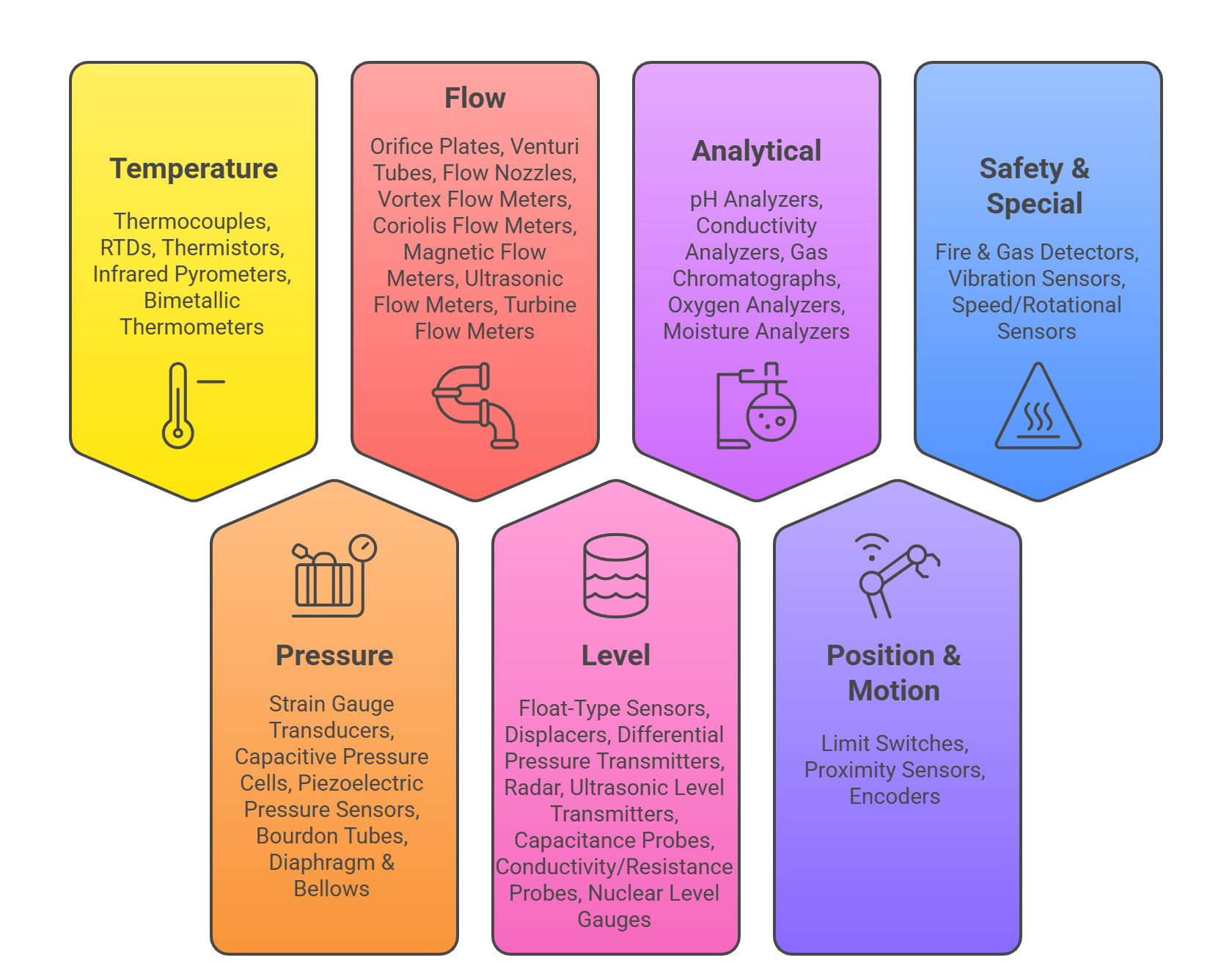
| Parameter | Instrument Types | Principle / Working |
|---|---|---|
| Temperature | Thermocouples | Generate voltage proportional to temperature difference (Seebeck effect). |
| Resistance Temperature Detectors (RTDs) | Electrical resistance changes with temperature. | |
| Thermistors | Semiconductor resistance varies non-linearly with temperature. | |
| Infrared Pyrometers | Detect thermal radiation from surfaces. | |
| Bimetallic Thermometers | Two metals expand differently causing mechanical movement. | |
| Pressure | Strain Gauge Transducers | Resistance changes when deformed under pressure. |
| Capacitive Pressure Cells | Capacitance changes with diaphragm deflection. | |
| Piezoelectric Pressure Sensors | Generate charge when stressed. | |
| Bourdon Tubes | Mechanical deflection due to pressure. | |
| Diaphragm & Bellows | Mechanical displacement under pressure. | |
| Flow | Orifice Plates | Differential pressure proportional to flow. |
| Venturi Tubes | Pressure differential in constricted flow section. | |
| Flow Nozzles | Similar to venturi, high-velocity measurement. | |
| Vortex Flow Meters | Detect vortices shed from bluff body. | |
| Coriolis Flow Meters | Mass flow measured via vibration frequency shift. | |
| Magnetic Flow Meters | Induced voltage proportional to fluid velocity. | |
| Ultrasonic Flow Meters | Transit-time or Doppler effect principle. | |
| Turbine Flow Meters | Rotor speed proportional to flow rate. | |
| Level | Float-Type Sensors | Mechanical float movement indicates level. |
| Displacers (Buoyancy) | Force on displacer changes with liquid level. | |
| Differential Pressure Transmitters | ΔP across tank height indicates level. | |
| Radar (FMCW / Pulse) | Time-of-flight of microwaves. | |
| Ultrasonic Level Transmitters | Echo time delay measurement. | |
| Capacitance Probes | Capacitance varies with liquid level. | |
| Conductivity/Resistance Probes | Detect conductive liquid contact. | |
| Nuclear Level Gauges | Gamma-ray attenuation indicates level. | |
| Analytical | pH Analyzers | Measure hydrogen ion activity. |
| Conductivity Analyzers | Measure ionic conductivity. | |
| Gas Chromatographs | Separate and measure gas components. | |
| Oxygen Analyzers | Electrochemical or paramagnetic measurement. | |
| Moisture Analyzers | Dew point or capacitance measurement. | |
| Position & Motion | Limit Switches | On/Off indication of valve position. |
| Proximity Sensors (Inductive/Capacitive) | Detect object presence. | |
| Encoders | Digital output proportional to shaft rotation. | |
| Safety & Special | Fire & Gas Detectors | IR/UV flame detection, catalytic/IR gas detection. |
| Vibration Sensors | Accelerometers for rotating equipment. | |
| Speed/Rotational Sensors | Magnetic or optical pickups. |
2.2.2 Transmitters: Signal Conversion and Communication
The raw signal generated by a sensor (e.g., a few millivolts from a thermocouple) is often weak, non-linear, and highly susceptible to electrical noise. It is unsuitable for transmission over long distances from the field to a central control room. This is where the Transmitter comes in.
A transmitter is an electronic device that takes the raw sensor signal, conditions it, linearizes it, and converts it into a standardized, robust industrial signal. This standardization is critical for ensuring interoperability between devices from different manufacturers. The most common analog standard is the 4–20 mA current loop.
In this system, 4 mA represents the lowest possible measurement (0% of scale) and 20 mA represents the highest (100% of scale). Digital communication protocols such as HART, Foundation Fieldbus, and Profibus are also widely used. Click to calculate 4 to 20 mA corresponding to 0% to 100%
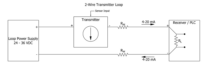
The distinction between a sensor and a transmitter is crucial. The sensor detects the physical variable, while the transmitter communicates that measurement in a standardized language. While modern instruments often integrate both into a single housing, understanding their separate functions is key to system design and troubleshooting. The 4–20 mA standard itself embodies a core principle of robust I&C design. By using 4 mA to represent the zero point of the measurement, the system can differentiate between a true zero reading and a fault condition like a broken wire, which would cause the current to drop to 0 mA. This concept, known as a “live zero,” provides an inherent, physical-layer diagnostic capability, making the transmitter a key element in ensuring system reliability.
2.2.3 Controllers: The System’s Brain
The standardized signal from the transmitter, representing the current value of the Process Variable, is sent to the Controller. The controller is the decision-making component—the “brain”—of the control loop.
Inside the controller, the incoming PV signal is continuously compared to the user-defined Setpoint (SP) to calculate the error.6 Based on this error value, the controller executes a pre-programmed control algorithm or logic to compute a corrective output signal. The most common algorithm used in industrial control is the Proportional-Integral-Derivative (PID) algorithm. The controller’s output signal, also typically in a standardized format like 4–20 mA, is then sent to the final element in the loop. Controllers can be implemented using various technologies, including standalone panel-mounted devices, Programmable Logic Controllers (PLCs), or as part of a large Distributed Control System (DCS).
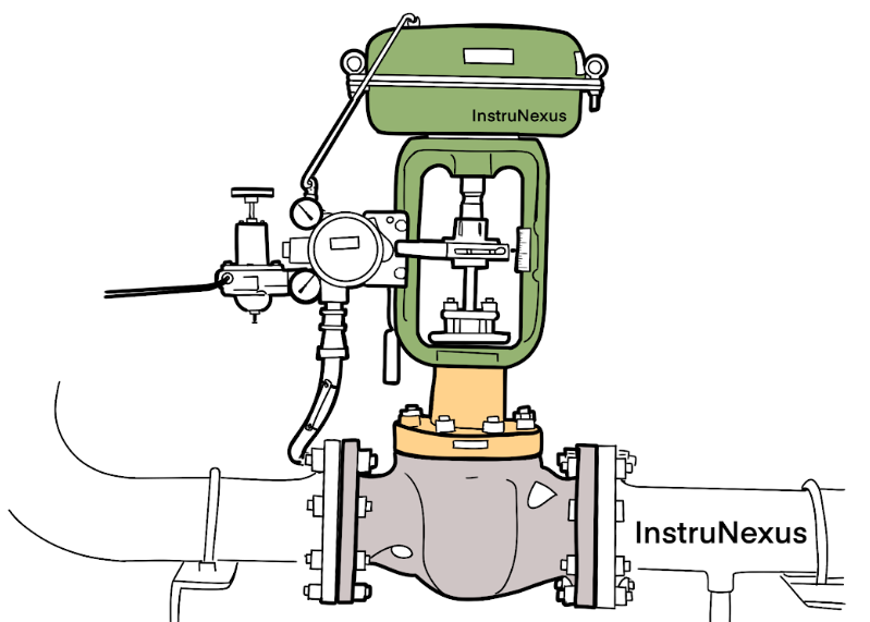
2.2.4 Final Control Elements (FCEs) and Actuators: The System’s Muscles
The controller’s output signal represents a decision, but it lacks the physical power to directly manipulate a large industrial process. The final stage of the loop translates this decision into physical action. This is the role of the Final Control Element (FCE) and its associated components. The FCE is the device that directly alters a manipulated variable in the process to bring the PV back toward the SP. It is often described as the “muscles” of the control loop.
Common examples of FCEs include:
- Control Valves: Used to regulate the flow of liquids or gases.
- Motors: Often paired with Variable Frequency Drives (VFDs) to control the speed of pumps, fans, or conveyors.
- Heating Elements: Used to control temperature.
- Dampers and Louvers: Used to control airflow in systems like HVAC or combustion processes.
The FCE is driven by an Actuator, which is the device that provides the motive force (e.g., pneumatic, electric, or hydraulic) to operate the FCE. For example, a pneumatic actuator uses compressed air to move the stem of a control valve. Often, a Transducer or Positioner is needed to convert the controller’s electrical signal (e.g., 4–20 mA) into the form of energy required by the actuator (e.g., a proportional pneumatic pressure of 3–15 psig).11 The positioner ensures the FCE moves to the exact position commanded by the controller, forming a small, fast control loop within the larger process loop.
2.3 Instrumentation Symbology: The Language of P&IDs
In professional practice, instrumentation and control systems are documented using a standardized graphical language on diagrams known as Piping and Instrumentation Diagrams (P&IDs). The Instrumentation, Systems, and Automation Society (ISA) has established a standard (ISA-5.1) for the symbols and identification codes used on these diagrams. Understanding this “shorthand” is essential for any I&C professional.
Instruments are typically represented by a circle (a “bubble”) containing a series of letters that identify the instrument’s function. The first letter denotes the measured process variable, and subsequent letters denote the function of the device.
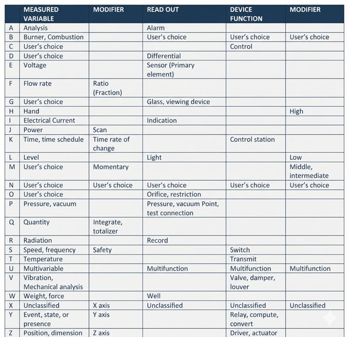
Adapted from ISA-5.1 standard information
For example, a device labeled TIC would be a Temperature Indicating Controller. A device labeled FT would be a Flow Transmitter. This standardized system allows engineers to convey complex control loop designs in a clear, concise, and universally understood format, bridging the gap between theoretical concepts and practical engineering documentation.
Part II: Control System Architectures and Strategies
The fundamental control loop provides the components for process regulation, but how these components are arranged and the logic they employ define the system’s overall architecture and strategy. The choice of architecture is a primary design decision that dictates the system’s accuracy, complexity, cost, and ability to handle disturbances. The most fundamental distinction is between open-loop and closed-loop control.
Section 3: Open-Loop vs. Closed-Loop Control
3.1 Open-Loop Systems: Principle, Examples, and Limitations
Principle: An open-loop control system, also known as a non-feedback system, is one in which the control action is completely independent of the process output. The system executes a predetermined set of instructions based on its input, without any mechanism to measure the result or compensate for deviations. It operates on a simple cause-and-effect basis: an input is given, and an action is performed, with no subsequent verification of the outcome.
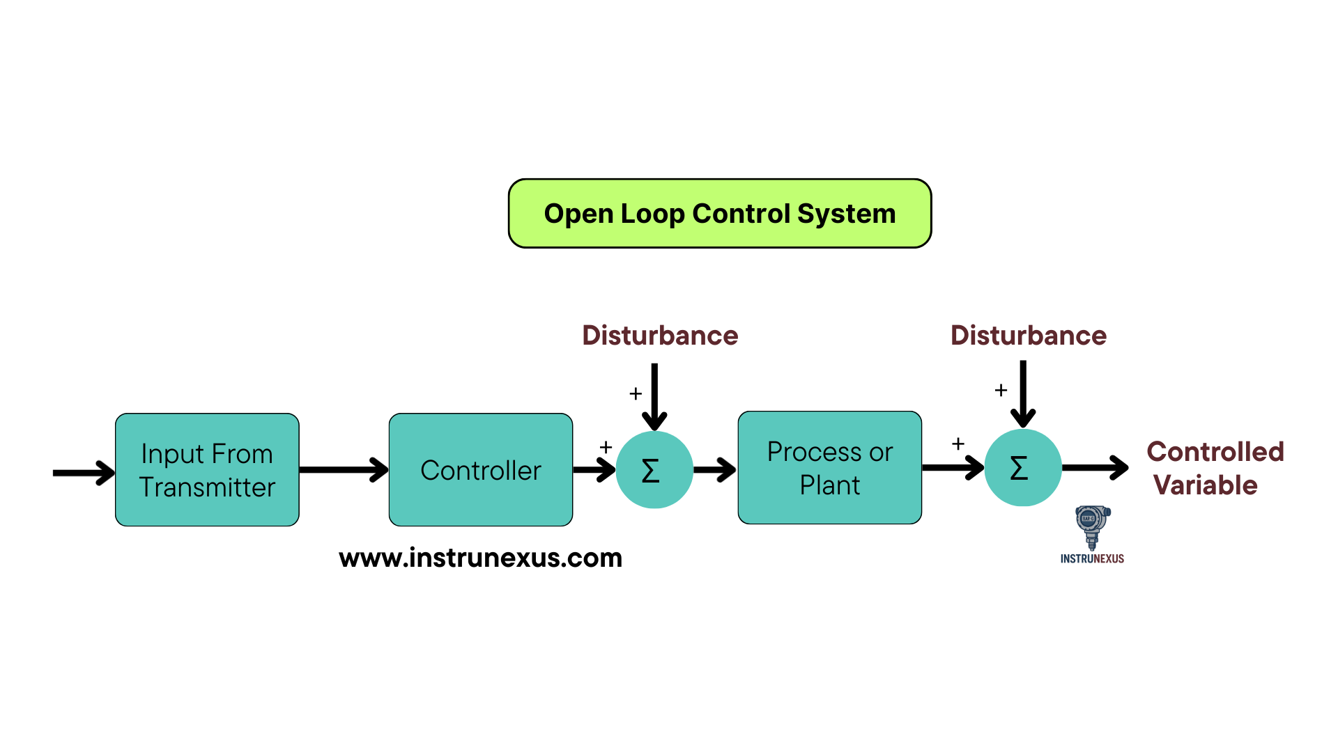
Examples: Open-loop systems are common in everyday devices and simple industrial applications where precision is not critical.
- A conventional toaster operates on a timer. It applies heat for a set duration, regardless of whether the bread is perfectly toasted or burnt.
- An automatic washing machine runs through a pre-programmed cycle of washing, rinsing, and spinning for a fixed time. It does not have sensors to check if the clothes are actually clean.21
- A simple immersion rod heater, when turned on, continuously supplies heat without monitoring the water temperature.
Advantages: The primary benefits of open-loop systems lie in their simplicity. They are:
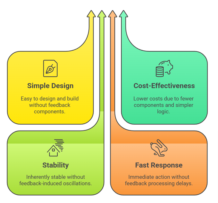
- Simple to Design and Build: The lack of feedback components makes their construction straightforward.
- Cost-Effective: Fewer components and simpler logic result in lower initial and maintenance costs.
- Inherently Stable: Since there is no feedback path, they cannot suffer from the instability or oscillations that can plague poorly tuned closed-loop systems.
- Fast Response: The action is immediate upon receiving an input, as there is no time delay for processing feedback signals.
Disadvantages: The lack of feedback is also their greatest weakness. Open-loop systems are:
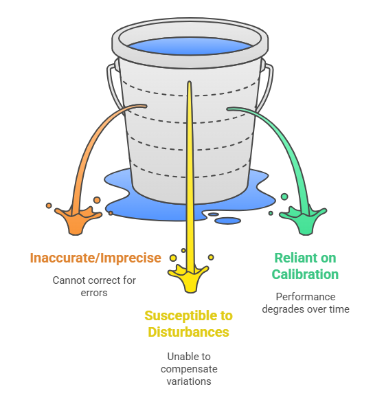
- Inaccurate and Imprecise: They cannot correct for errors or deviations from the desired outcome.
- Susceptible to Disturbances: They are unable to compensate for external disturbances or internal variations in the process (e.g., a drop in voltage affecting a heater’s output).
- Reliant on Calibration: Their performance is entirely dependent on the accuracy of their initial calibration. Any change in the system over time will lead to performance degradation.
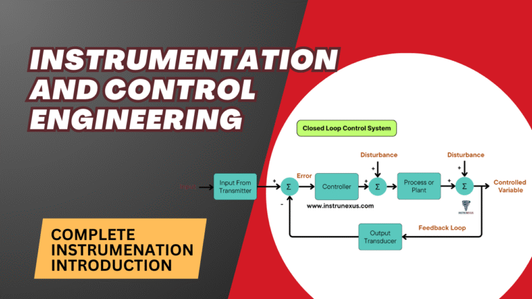
3.2 Closed-Loop Systems: The Power of Feedback
Principle: A closed-loop control system, or feedback system, is defined by its use of feedback. It continuously measures the actual process output (the PV) and feeds this information back to the controller. The controller then compares this measured output to the desired setpoint (SP) and automatically adjusts its control action to minimize the difference, or error. This continuous loop of measurement, comparison, and correction is the hallmark of modern automated control and is the basis for most industrial control systems.
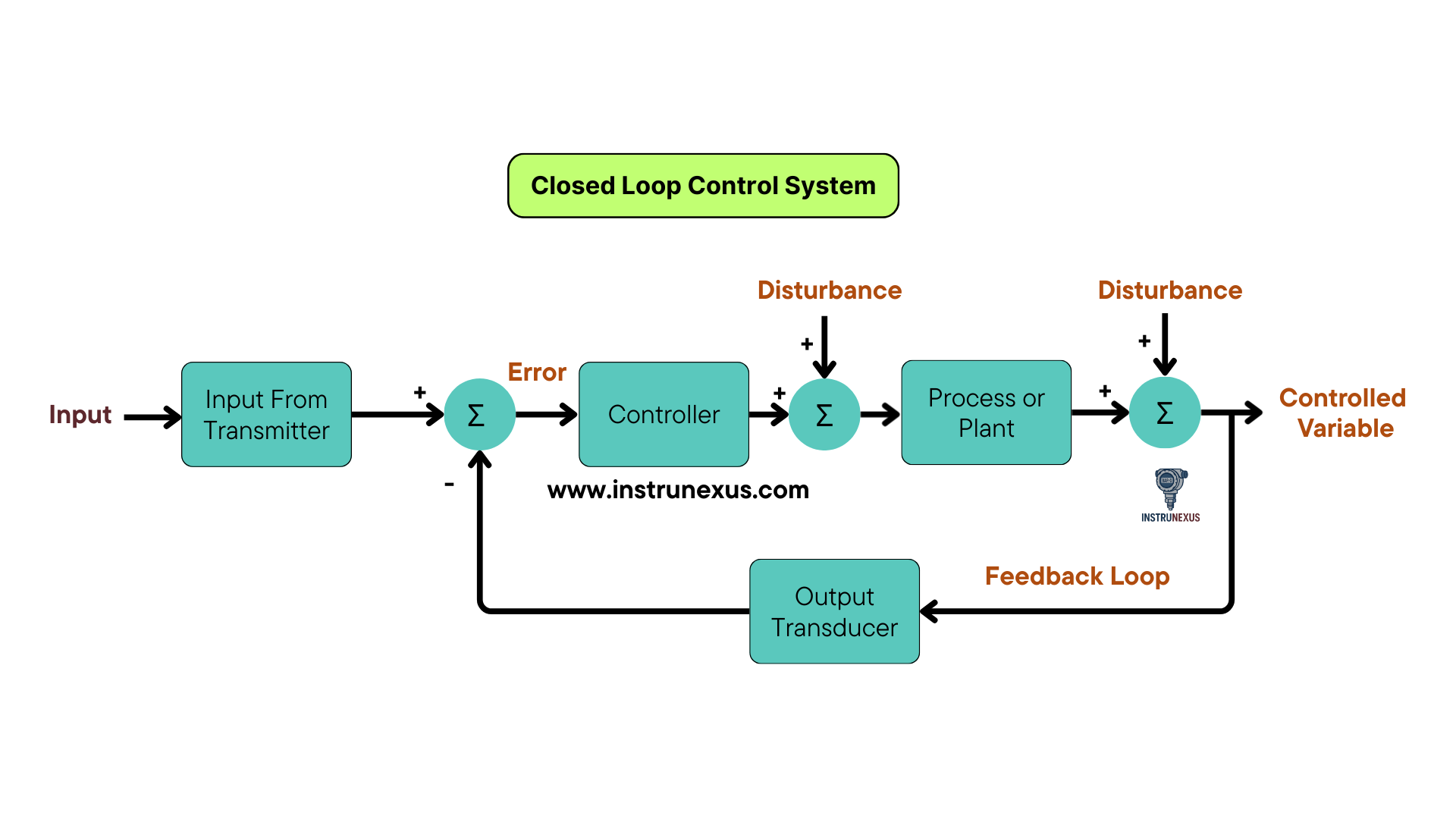
Examples: Closed-loop systems are ubiquitous in applications where accuracy and adaptability are required.
- A home thermostat continuously measures the room temperature (PV). If it falls below the setpoint (SP), the controller signals the furnace to turn on. When the temperature reaches the setpoint, it signals the furnace to turn off.
- The cruise control in an automobile measures the vehicle’s speed. If the car slows down while going up a hill, the controller increases the engine’s throttle to bring the speed back to the setpoint.
- In an industrial setting, a level controller in a tank measures the liquid level and adjusts an inflow valve to maintain that level despite variations in the outflow rate.
Advantages: The benefits of closed-loop control are significant and are the reason for its widespread use in industry. They offer:
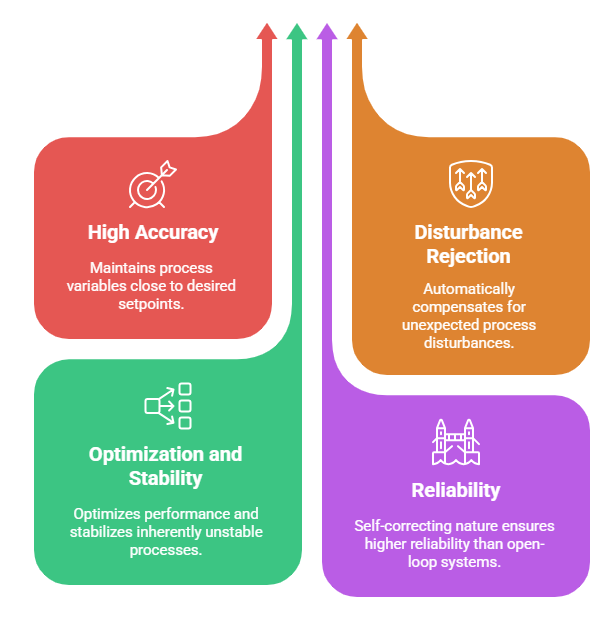
- High Accuracy: By continuously correcting for errors, they can maintain the process variable very close to the setpoint.
- Disturbance Rejection: They can automatically compensate for unexpected disturbances, making the process robust and stable.
- Optimization and Stability: They can be used to optimize process performance and even stabilize processes that are inherently unstable.
- Reliability: The self-correcting nature makes them more reliable than open-loop systems.
Disadvantages: The added complexity of feedback systems introduces its own set of challenges. They are:
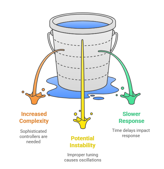
- More Complex and Costly: The need for sensors, transmitters, and more sophisticated controllers makes them more complex and expensive to design and implement.
- Potential for Instability: The feedback loop introduces the possibility of oscillations or instability if the controller is not properly tuned. An overly aggressive controller can “overreact” to errors, causing the process variable to swing wildly around the setpoint.
- Slower Response: The time required to measure the PV, feed it back, and process the control calculation can result in a slightly slower initial response compared to an open-loop system.
3.3 A Comparative Analysis: When to Use Each System
The decision to use an open-loop or closed-loop architecture depends on a careful analysis of the process requirements, the nature of potential disturbances, and budget constraints.
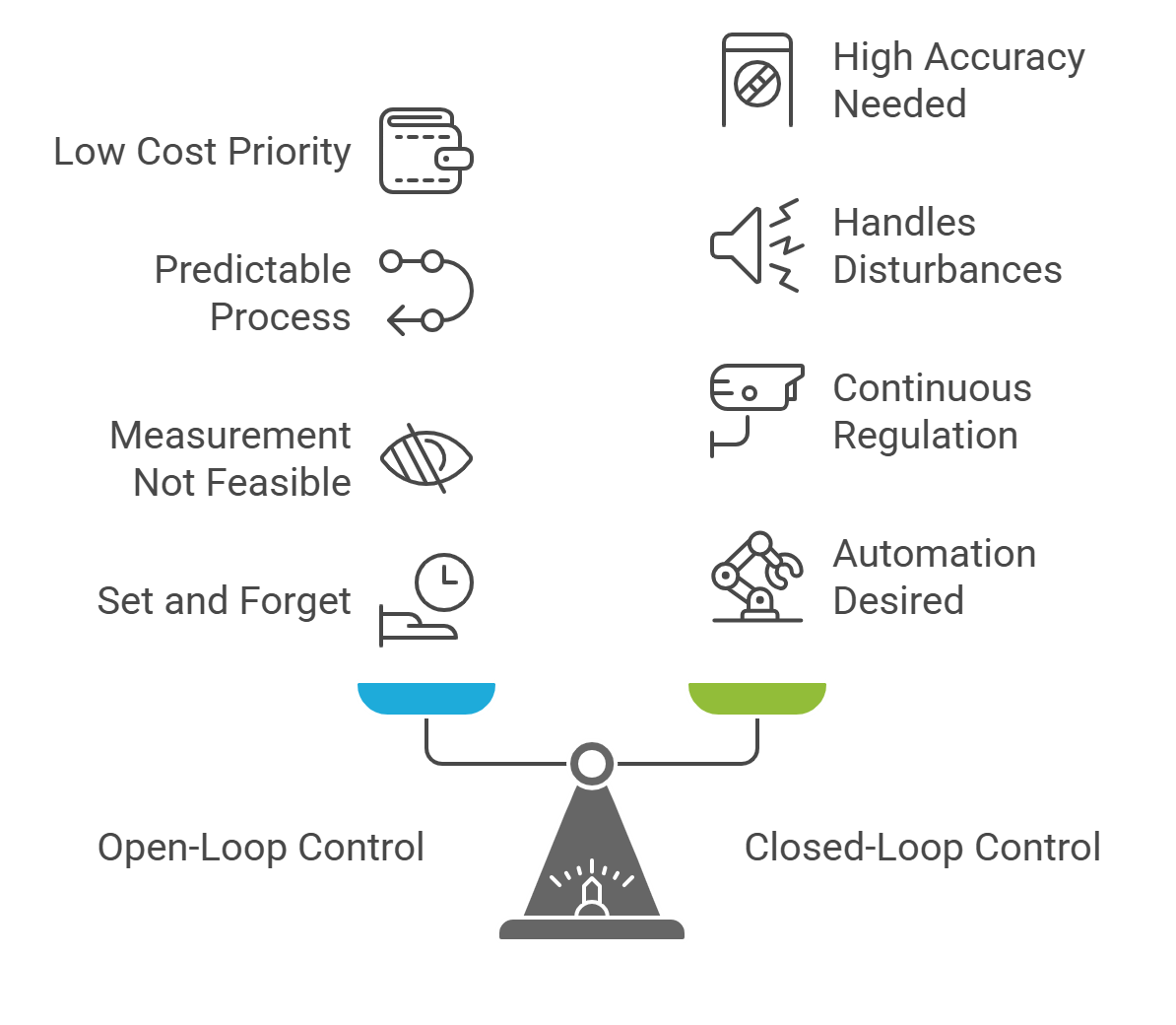
Use Open-Loop control when:
- Low Cost is a Priority: For simple, non-critical applications where the cost of a feedback system is prohibitive.
- The Process is Highly Predictable: For systems where the relationship between input and output is well-known and stable, and disturbances are rare or insignificant.
- Measurement is Not Feasible: In cases where it is impossible or impractical to measure the output variable quantitatively.
- The Output Rarely Changes: For “set and forget” applications like turning on a cooling pump that runs continuously.
Use Closed-Loop control when:
- Accuracy is Critical: In any process where maintaining a precise setpoint is essential for product quality, safety, or efficiency.
- Disturbances are Expected: For processes that are subject to variations in load, ambient conditions, or raw material properties.
- The Process is Not “Set and Forget”: When the output variable is expected to change and requires continuous regulation.
- Automation is Desired: While more expensive than open-loop hardware, automated closed-loop systems are often significantly less expensive than employing human operators for continuous manual adjustment.
3.4 Summary Comparison
The fundamental differences between these two control architectures are summarized in the table below.
Basis of Difference | Open-Loop Control System | Closed-Loop Control System |
Feedback Path | Absent. The control action is independent of the output. | Present. The control action is dependent on the measured output. |
Control Philosophy | Pre-programmed, non-adaptive. | Adaptive, self-correcting. |
Complexity & Cost | Simple design, less expensive, easier to build and maintain. | Complex design, more expensive, more difficult to implement. |
Accuracy & Reliability | Less accurate and less reliable. Performance depends on calibration. | Highly accurate and more reliable due to error correction. |
Response to Disturbances | Cannot compensate for disturbances or process variations. | Automatically corrects for disturbances. |
Stability | Generally more stable, as it cannot oscillate due to feedback. | Can become unstable or oscillate if not properly tuned. |
Response Speed | Fast initial response. | Slower response due to feedback processing time. |
Typical Examples | Toaster, traffic light, automatic washing machine. | Thermostat, cruise control, industrial process controllers. |
Section 4: Advanced Disturbance Rejection Strategies
While standard feedback control is a powerful tool, complex industrial processes often present challenges—such as significant time delays and large, predictable disturbances—that require more sophisticated strategies. Feedforward and cascade control are two advanced architectures designed to overcome the limitations of simple feedback by using additional process information to improve stability and responsiveness. The progression from feedback to these advanced strategies represents an evolution in how control systems utilize information and manage time.
4.1 Feedback Control: Correcting for Error
As established, standard feedback control is a reactive strategy. The controller’s action is triggered only after a disturbance has already affected the process and caused the Process Variable (PV) to deviate from the Setpoint (SP), creating an error. It operates by observing information from the past (the error that has already occurred) to make a correction in the present.
The primary strength of this approach is its universality. A feedback controller will attempt to correct for any disturbance that impacts the measured PV, regardless of the disturbance’s source or nature. This makes it robust against unmeasured or unknown process upsets. Furthermore, when integral action is included in the controller, it ensures that the system will eventually return precisely to the setpoint, eliminating any permanent offset. However, its reactive nature means that for processes with long delays, the disturbance may cause a significant deviation before the controller’s corrective action can take effect.
4.2 Feedforward Control: Anticipating Disturbances
Feedforward control is a proactive or predictive strategy. Instead of waiting for an error to appear in the PV, it measures a major, known disturbance variable directly, before it has a chance to significantly impact the process. It uses information about the
present state of a disturbance to predict its effect on the future state of the process and deploys a preemptive control action to counteract it.
Architecture: A feedforward system requires two key elements: a sensor to measure the disturbance variable, and a mathematical model of the process that predicts how a change in the disturbance will affect the PV. The feedforward controller uses this model to calculate the exact change needed in the manipulated variable to cancel out the impending effect of the disturbance.
Example: Consider a heat exchanger where the goal is to maintain the outlet temperature of a process fluid (PV) by manipulating the flow of steam (manipulated variable). A major disturbance could be a change in the inlet flow rate of the process fluid. A feedforward controller would measure this inlet flow rate (the disturbance). If the flow rate increases, the controller knows this will cause the outlet temperature to drop. Using its process model, it preemptively increases the steam flow to add more heat, counteracting the disturbance before the outlet temperature has a chance to deviate significantly from its setpoint.
Limitations and Implementation: The major limitation of pure feedforward control is its reliance on a perfect model and its inability to handle unmeasured disturbances. Any inaccuracy in the model or any other upset to the process will result in an error that the feedforward controller cannot see or correct. For this reason, feedforward control is almost never used alone in industrial practice. It is typically combined with a standard feedback loop in an architecture known as feedforward with feedback trim. In this arrangement, the feedforward controller makes the primary, proactive corrections for the major measured disturbance, while the feedback controller acts as a “trim,” correcting for any residual error caused by model inaccuracies or other, unmeasured disturbances.
For detailed Feedforward controllers click here
4.3 Cascade Control: Nested Loops for Enhanced Stability
Cascade control is a strategy of “divide and conquer.” It is designed for processes that have a slow-responding primary variable but also contain a faster-responding intermediate variable that is influenced by the same manipulated input. It improves disturbance rejection by tackling upsets at a faster, more localized level before they can propagate to the slower main process.
Principle: A cascade control system consists of two nested feedback loops: a primary (or master) loop and a secondary (or slave) loop.
- The primary controller measures the final, slow-responding PV (e.g., reactor temperature) and compares it to the ultimate setpoint.
- The output of the primary controller is not sent directly to the final control element. Instead, it becomes the setpoint for the secondary controller.
- The secondary controller measures a faster-responding intermediate process variable (e.g., the temperature of the heating jacket fluid) that has a direct and rapid influence on the primary PV.
- The secondary controller then manipulates the final control element (e.g., the steam valve to the jacket) to keep the intermediate variable at the setpoint provided by the primary controller.
Purpose and Requirements: The purpose of this arrangement is to isolate the slow primary loop from disturbances that affect the faster secondary loop.35 For example, if the steam supply pressure fluctuates, this will immediately affect the jacket temperature. The fast secondary loop will instantly detect this and correct the steam valve position to stabilize the jacket temperature, all before the fluctuation has time to significantly impact the much slower-reacting bulk temperature inside the reactor. This makes the overall control of the primary variable much smoother and more stable. An essential requirement for cascade control to be effective is that the
secondary loop must respond significantly faster than the primary loop.
Example: A common industrial application is a boiler feedwater control system. The primary goal is to maintain the water level in the steam drum (a slow process). The primary level controller measures the drum level. Its output sets the setpoint for a secondary flow controller, which measures the flow rate of feedwater into the boiler (a very fast process). If the feedwater supply pressure drops (a disturbance), the flow controller will immediately open the feedwater valve further to maintain the required flow rate, correcting the problem long before the drum level begins to drop noticeably. The primary level controller is thus shielded from this common and rapid disturbance.
The choice between these advanced strategies depends on a deep understanding of the physical process. If a major disturbance is measurable and its effect is predictable, feedforward control is a powerful option. If the process contains a suitable, fast-acting intermediate variable, cascade control can provide exceptional stability. These strategies demonstrate that effective control system design is not just about applying algorithms, but about intelligently structuring the flow of information to best manage the specific dynamics and challenges of the process being controlled.
For detailed Cascade controllers click here
Section 5: The Proportional-Integral-Derivative (PID) Algorithm
At the heart of the vast majority of closed-loop control systems lies a remarkably effective and enduring algorithm: the Proportional-Integral-Derivative (PID) controller. First developed in the early 20th century and formalized for industrial use by the 1940s, the PID algorithm is the workhorse of process control due to its relative simplicity, robustness, and ability to provide precise and stable control for a wide variety of processes. It operates by calculating a controller output based on three distinct terms derived from the process error: a term based on the present error, a term based on the accumulation of past error, and a term based on the prediction of future error.
5.1 The Mathematical Foundation of PID Control
The PID controller continuously calculates an error value, e(t), as the difference between the desired Setpoint (SP) and the measured Process Variable (PV): e(t)=SP−PV. It then computes a corrective output signal,
u(t), which is sent to the final control element. This output is the sum of the three control terms: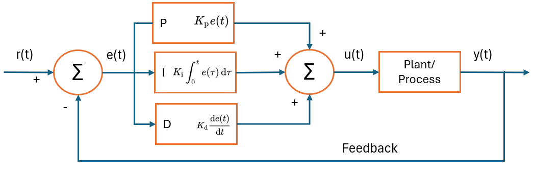
u(t)=Kp e(t)+Ki∫0te(τ) dτ+Kd dt de(t)
In this standard “textbook” equation
- Kp is the Proportional Gain.
- Ki is the Integral Gain.
- Kd is the Derivative Gain.
These three user-adjustable parameters, known as the controller gains, are “tuned” to match the specific response characteristics of the process being controlled. In many industrial controllers, the parameters are expressed in a dependent form using a controller gain (Kc), an integral time or reset time (τI), and a derivative time (τD). While the formulation may differ, the underlying principle of combining proportional, integral, and derivative actions remains the same.
5.2 The Role of the Proportional (P) Term: Present Error Response
The proportional term produces an output that is directly proportional to the magnitude of the current error.13 It provides an immediate, scaled response to any deviation from the setpoint.
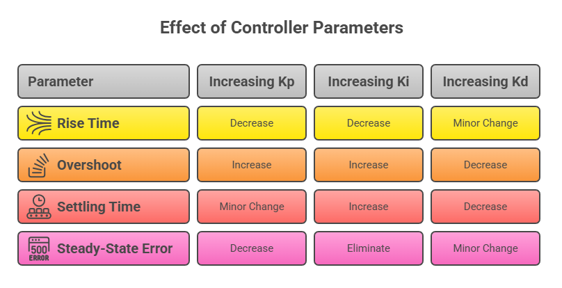
Effect: The proportional gain, Kp, determines the aggressiveness of this response. A higher Kp will result in a larger change in the controller output for a given error, causing the system to react more quickly. However, this increased aggressiveness comes at a cost. As Kp is increased, the tendency for the process variable to overshoot the setpoint also increases. If the gain is set too high, the system can become unstable and begin to oscillate uncontrollably.
A critical characteristic of a controller using only proportional action (a P-only controller) is that it will almost always exhibit a steady-state error, also known as offset. This is because for the controller to produce a non-zero output to hold the process against a steady load, there must be a non-zero error. An equilibrium is reached where the error is just large enough to generate the output needed to maintain the process at a stable value, which will be offset from the setpoint.
5.3 The Role of the Integral (I) Term: Eliminating Steady-State Error
The integral term is designed to eliminate the steady-state error inherent in P-only control. It works by looking at the history of the error, summing or integrating the error value over time.
Effect: As long as any error persists, no matter how small, the integral term will continuously accumulate, causing the controller output to gradually increase or decrease. This continues until the error is driven to zero, at which point the integral term stops changing and holds its value, providing the necessary output to keep the PV at the SP. The integral gain,
Ki, determines how quickly the integral action accumulates.
While essential for accuracy, the integral term can have negative effects on stability. It tends to increase overshoot and can slow down the system’s response to disturbances. A significant issue associated with integral action is integral windup. This occurs when a large change in setpoint causes a large, prolonged error. The integral term accumulates to a very high value, saturating the controller output (e.g., driving a valve fully open). When the PV finally approaches the SP, the large accumulated value in the integrator keeps the output saturated, causing a massive overshoot. Anti-windup strategies are often employed in commercial controllers to mitigate this effect.
5.4 The Role of the Derivative (D) Term: Predicting Future Error
The derivative term provides an “anticipatory” or damping action by looking at the rate of change of the error.13 It predicts the future trend of the error based on its current slope.
Effect: If the process variable is moving rapidly toward the setpoint, the error is decreasing quickly. The derivative term will produce an opposing control action to “put the brakes on,” slowing the approach to the setpoint. This action effectively adds damping to the system, which serves to reduce overshoot and settle the system more quickly after a disturbance or setpoint change.39 The derivative gain,
Kd, determines the strength of this damping effect.
The primary drawback of the derivative term is its extreme sensitivity to measurement noise. High-frequency noise in the sensor signal can cause large, rapid fluctuations in the calculated derivative, leading to an erratic and “jumpy” controller output that can cause excessive wear on final control elements and even destabilize the loop.39 For this reason, the derivative term is used less frequently than the P and I terms, and many industrial control loops are successfully run as PI controllers. When D-action is used, the signal is often heavily filtered, or the calculation is based on the rate of change of the PV rather than the error to avoid “derivative kick” on sudden setpoint changes.39
5.5 Practical Guide to Loop Tuning: Methods and Considerations
Loop tuning is the process of methodically adjusting the P, I, and D gain parameters to achieve an optimal control response for a specific process. The goal is to find a balance between responsiveness and stability—a response that is fast without excessive overshoot or oscillation.
Manual Tuning Method: A common hands-on approach involves the following steps:
- Start with P-only control: Set the integral (Ki) and derivative (Kd) gains to zero.
- Increase Proportional Gain: With the controller in automatic mode, make a small step change to the setpoint. Gradually increase the proportional gain (Kp) and repeat the step change until the process variable begins to oscillate with a constant amplitude. This gain value is known as the ultimate gain (Ku).
- Measure Oscillation Period: Measure the time period of one full oscillation. This is the ultimate period (Pu).
- Calculate Gains: Use the measured Ku and Pu values in established formulas, such as those from the Ziegler-Nichols method, to calculate initial values for Kp, Ki, and Kd.
- Fine-Tune: Make small adjustments to the calculated gains to optimize the response for the specific application, balancing speed, overshoot, and settling time.
Ziegler-Nichols Method: This is a more formalized version of the manual tuning process that provides specific formulas for calculating the PID gains based on the experimentally determined Ku and Pu. While widely known, it often produces aggressive tuning that may need to be detuned for practical applications.
Tuning a PID controller is both a science and an art, requiring an understanding of the process dynamics and the effect of each control term. The optimal tuning is always a compromise tailored to the specific goals of the process, whether that is rapid response, minimal overshoot, or robust disturbance rejection.
5.6 Summary of PID Term Effects
The qualitative effects of independently increasing each gain parameter on the closed-loop response are summarized below. This table serves as a valuable reference guide for manual tuning.
Part III: Industrial Implementation and Applications
The theoretical principles of control loops and algorithms are brought to life through a range of specialized industrial technologies. The choice of technology is dictated by the specific demands of the application, including the type of process, its scale, and its geographical distribution. This section explores the primary hardware and software platforms used for industrial control—PLCs, DCS, and SCADA—and then examines their application in key industrial sectors.
Section 6: Key Industrial Control Technologies
While modern systems often blend functionalities, the three primary categories of industrial control systems—Programmable Logic Controllers (PLCs), Distributed Control Systems (DCS), and Supervisory Control and Data Acquisition (SCADA) systems—were each designed with a distinct philosophy and purpose. Understanding these core design intentions is crucial for selecting the appropriate technology for a given task. The choice is fundamentally driven by the nature of the process (discrete vs. continuous), its physical scale (a single machine vs. an entire plant vs. a widespread enterprise), and its geographical layout (local vs. dispersed).
6.1 Programmable Logic Controllers (PLCs): Architecture and Discrete Control
Definition: A Programmable Logic Controller (PLC) is a ruggedized, solid-state industrial computer designed specifically for the control of manufacturing processes. They were originally developed in the automotive industry in the late 1960s to replace inflexible and maintenance-intensive hard-wired relay panels. A PLC is a hard real-time system, meaning it must produce output results in response to input conditions within a bounded time to ensure safe and predictable operation.
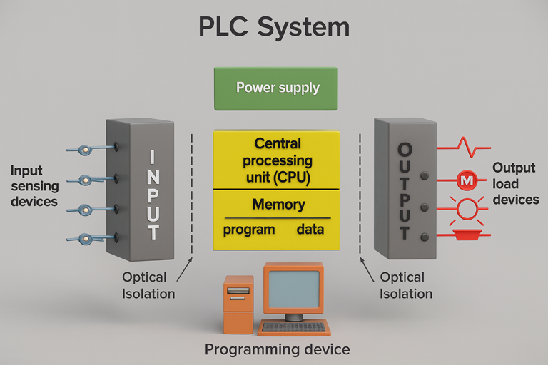
Architecture: A PLC system is composed of several key components:
- Central Processing Unit (CPU): The brain of the PLC, which executes the user-programmed logic, processes data, and manages communications.
- Memory: Includes ROM for the operating system and RAM for the user program and data. Programs are typically stored in non-volatile or battery-backed memory to prevent loss during a power failure.
- Power Supply: Converts standard AC voltage to the low-voltage DC required by the PLC’s internal components.
- Input/Output (I/O) Modules: These are the interface to the physical world. Input modules receive signals from field devices like switches, sensors, and pushbuttons. Output modules send signals to control devices like motors, solenoids, and indicator lights.46 I/O can be digital (discrete on/off signals) or analog (variable signals like 4–20 mA).
- Mechanical Form Factor: PLCs come in two main styles: compact or “brick” PLCs, which integrate the CPU, power supply, and a fixed number of I/O into a single housing, and modular PLCs, which use a rack or chassis system where individual modules for the CPU, power supply, and various types of I/O can be mixed and matched for greater flexibility and expandability.
Operation and Programming: PLCs operate on a repetitive process called the scan cycle. In each cycle, the PLC reads the status of all inputs, executes the user program from top to bottom, and then updates the status of all outputs accordingly. This cycle is repeated continuously at very high speeds. PLCs are designed to be programmed by engineers and technicians who may not have formal computer science backgrounds. The most common programming language is Ladder Logic (LAD), a graphical language that visually resembles the relay logic diagrams it was designed to replace. Other standard languages include Function Block Diagram (FBD) and Structured Text (ST).
Primary Application: PLCs excel at high-speed, bit-level logic and sequential control. Their core strength lies in discrete manufacturing and machine automation, such as controlling assembly lines, packaging machines, robotic cells, and conveyor systems. While fully capable of performing analog control and executing PID loops, their fundamental design is optimized for fast, deterministic, logic-based control.
6.2 Distributed Control Systems (DCS): Architecture and Large-Scale Process Management
Definition: A Distributed Control System (DCS) is a computerized control system for a large-scale process or plant, characterized by the distribution of autonomous controllers throughout the system, all connected via a high-speed communication network. Unlike a centralized system that relies on a single computer, a DCS distributes the control processing, which significantly enhances reliability.
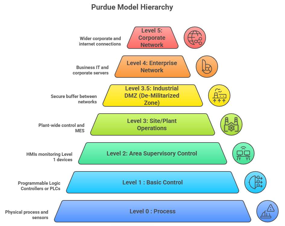
Architecture: The architecture of a DCS is hierarchical and distributed :

- Level 0 (Field Level): This level contains the field devices, such as sensors and final control elements (valves, actuators).
- Level 1 (Control Level): This level consists of the distributed controllers (or process control units). Each controller is responsible for a specific section of the plant and contains its own processor and I/O modules to handle a subset of the plant’s control loops. This localization of control processing near the equipment ensures fast response times and means that the failure of a single controller will only affect its designated area, not the entire plant.
- Level 2 (Supervisory Level): This level includes the supervisory computers, which are located in a central control room. These computers gather data from all the distributed controllers and provide the Human-Machine Interface (HMI) for the plant operators. From these workstations, operators can monitor the entire process, view trends, respond to alarms, and change setpoints.
- Higher Levels (Production Control & Scheduling): Levels 3 and 4 interface with plant-wide business systems for production planning and scheduling.
Operation and Programming: A DCS is process-oriented rather than machine-oriented. It is designed from the ground up to handle complex, multi-variable analog control strategies like cascade loops and interlocks in an integrated fashion. Programming is often done using function blocks, where pre-defined algorithms (like PID controllers, summers, filters) are graphically linked together to build a control strategy. The system provides a unified database and a cohesive environment for control configuration, HMI development, and data historization.
Primary Application: DCS are the preferred solution for large-scale, continuous or batch process industries where high reliability, process stability, and integrated plant-wide control are paramount. They are found in industries such as oil and gas refining, chemical and petrochemical manufacturing, pulp and paper, and power generation.
6.3 Supervisory Control and Data Acquisition (SCADA): High-Level Supervision for Geographically Dispersed Operations
Definition: SCADA is a system architecture designed for high-level monitoring and control of processes that are spread over large geographical areas.57 Its primary focus is on data acquisition from remote locations and providing a centralized supervisory overview.
Architecture: A typical SCADA system consists of :
- Master Terminal Unit (MTU) or SCADA Server: A central computer or server that hosts the SCADA software, communicates with remote sites, and provides the HMI for operators.
- Remote Terminal Units (RTUs) or PLCs: These devices are located at the remote sites. They interface directly with local sensors and actuators, collect data, and can perform local control functions. They transmit data back to the master station and execute commands received from it.
- Communications Network: This is a critical component, as it links the central master station with the numerous remote sites. Unlike the high-speed, reliable local area networks (LANs) used in a DCS, SCADA systems often have to rely on a variety of communication media, including telephone lines, cellular networks, radio, microwave, and satellite, which can have higher latency and lower reliability. This influences the system’s design, which often uses a poll-response communication method.
Operation and Philosophy: The philosophy of SCADA is supervisory. While RTUs can perform local closed-loop control, the system’s main function is to provide operators at a central location with the ability to monitor remote assets, gather data for analysis, and issue high-level commands (e.g., open or close a pipeline valve, change a setpoint on a remote controller). The real-time control is often less continuous and high-speed compared to a DCS.
Primary Application: SCADA is the ideal technology for industries with geographically dispersed infrastructure. Common applications include:
- Oil and Gas: Monitoring and controlling pipelines, wellheads, and pumping stations spread over hundreds of miles.
- Electrical Power: Managing transmission and distribution grids.
- Water and Wastewater: Controlling water distribution networks, treatment plants, and remote pumping stations.
- Transportation: Managing railway systems or traffic light networks.
While the historical distinctions are clear, modern technology has led to a significant convergence of capabilities. High-end PLCs now have powerful process control and networking features, DCS platforms can incorporate PLC-style logic for discrete control, and SCADA systems are being built on faster, more reliable networks, allowing them to perform more like a DCS. A modern industrial facility might employ a hybrid architecture: PLCs controlling individual machines, which are integrated into a plant-wide DCS for overall process management, with a SCADA system linking multiple facilities to a corporate headquarters for enterprise-level monitoring.
6.4 Comparative Analysis of PLC, DCS, and SCADA Systems
Characteristic | Programmable Logic Controller (PLC) | Distributed Control System (DCS) | Supervisory Control and Data Acquisition (SCADA) |
Primary Process Type | Discrete (On/Off), Sequential | Continuous, Batch | Supervisory, Data Acquisition |
Typical Application | Machine control, assembly lines, robotics | Chemical plants, refineries, power plants | Pipelines, power grids, water distribution |
System Scale | Machine, Small Unit | Plant-wide | Enterprise-wide, Multiple Sites |
Geographical Distribution | Localized | Localized within a plant site | Geographically Dispersed |
Control Philosophy | Logic-based, fast execution | Process-oriented, integrated control | Supervisory, remote monitoring and command |
Response Speed | Very Fast (milliseconds) | Fast (sub-second) | Slower (seconds to minutes), dependent on comms |
Redundancy | Available, but often optional | Integral to the design, high reliability | Often designed into master station and comms |
Cost | Lower cost per I/O point | Higher initial system cost | Varies greatly with scale and comms infrastructure |
Section 7: Applications in the Process Industries
The theoretical frameworks and technological platforms of instrumentation and control find their ultimate value in their application to real-world industrial processes. In the process industries, such as chemical and pharmaceutical manufacturing, I&C systems are not merely tools for efficiency but are fundamental to ensuring product quality, operational safety, and regulatory compliance.
7.1 Chemical Processing: A Case Study in Reactor Temperature and pH Control
Context: The chemical industry relies on the precise manipulation of chemical reactions to transform raw materials into valuable products. Control systems are a transformative force in this sector, providing the means to enhance process efficiency, improve safety standards, facilitate quality assurance, and optimize resource management. The meticulous regulation of critical process variables like temperature, pressure, flow, and pH is essential for maximizing reaction yield, ensuring product consistency, and preventing hazardous runaway conditions.
Application Example: Temperature and pH Control in a Jacketed Reactor
A jacketed reactor is a common piece of equipment in chemical processing, consisting of an inner vessel where the reaction takes place and an outer jacket through which a thermal fluid is circulated to control the reaction temperature. Maintaining precise temperature and, in many cases, pH is critical to the success of the reaction.
- Instrumentation:
- A temperature sensor (e.g., an RTD or thermocouple) is installed inside the reactor to provide a continuous measurement of the reaction mixture’s temperature (the primary PV).
- Additional temperature sensors may be placed on the jacket inlet and outlet to monitor the thermal fluid.
- For pH-sensitive reactions, a pH probe is inserted into the reactor to measure the acidity or alkalinity of the mixture.
- Sensors for other variables like pressure or stirring speed may also be included.
- Control System:
- An automated controller, which could be part of a DCS or a dedicated reactor control system, receives the signals from all the sensors.
- The controller executes a control strategy, often a cascade loop. The primary (master) controller compares the reactor temperature to the desired setpoint. Its output becomes the setpoint for a secondary (slave) controller that regulates the temperature of the jacket fluid.
- Simultaneously, a separate control loop compares the measured pH to its setpoint.
- Final Control Elements:
- The secondary temperature controller manipulates the final control elements for heat transfer. This typically involves a control valve that regulates the flow of a heating medium (like steam) or a cooling medium (like chilled water) into the jacket. A pump circulates the fluid through the jacket.
- The pH controller manipulates one or more dosing pumps, which precisely add an acid or base reagent to the reactor to maintain the pH at its setpoint.
Benefits: This automated control scheme provides significant advantages over manual operation. By maintaining constant and precise temperature and pH control throughout the entire reaction, the system can achieve higher yields and better selectivity, minimizing the formation of undesirable by-products. Real-time monitoring of equipment parameters enables predictive maintenance, reducing downtime. Most importantly, the automation enhances safety by ensuring the reaction stays within its safe operating envelope and by reducing the need for direct human interaction with potentially hazardous processes.
7.2 Pharmaceutical Manufacturing: Ensuring Quality and Compliance
Context: The pharmaceutical and biotechnology industries operate under some of the most stringent regulatory frameworks in the world, such as the Good Manufacturing Practice (GMP) guidelines enforced by agencies like the U.S. Food and Drug Administration (FDA). In this environment, instrumentation and control systems are indispensable for ensuring product quality, process consistency, data integrity, and ultimately, patient safety. Every instrument that has a direct impact on product quality must be meticulously calibrated and maintained.
Application Example: Fermentation Process Optimization
In biopharmaceutical manufacturing, fermentation or cell culture is a critical upstream process where microorganisms or mammalian cells are grown to produce a desired therapeutic protein. The health and productivity of these cultures are extremely sensitive to their environmental conditions.
- Instrumentation: To gain deep insight into the metabolic state of the culture, advanced instrumentation is used. For example, an online process mass spectrometer can be connected to the fermenter’s exhaust gas line to provide real-time, high-precision measurements of oxygen (O2) consumption and carbon dioxide (CO2) evolution. This allows for the calculation of the Respiratory Quotient (RQ), a key indicator of metabolic activity. Highly reliable and self-calibrating temperature sensors are also critical.
- Control and Benefits: This real-time data is fed into the control system (typically a DCS). By monitoring the RQ, operators and automated control strategies can take immediate corrective action—such as adjusting the feed rate of nutrients or the aeration rate—to optimize the culture’s health and productivity. This level of control prevents the loss of entire high-value fermentation batches, which can take weeks to run and cost a significant amount in media and labor.
Application Example: Real-Time Quality Control (QC)
Traditional QC in pharmaceutical manufacturing involves taking samples from the production line and sending them to a centralized laboratory for analysis using time-consuming methods like High-Performance Liquid Chromatography (HPLC) or Gas Chromatography (GC). This creates significant delays and production bottlenecks.67
- Instrumentation and Control: A modern approach, aligned with the FDA’s Process Analytical Technology (PAT) initiative, is to implement at-line or in-line analysis using advanced instrumentation. For instance, a handheld Raman spectroscopy analyzer can be used directly on the manufacturing floor to perform tasks like:
- Raw Material Identification: Verifying the identity and quality of incoming raw materials in seconds, right at the receiving dock.
- In-Process Monitoring: Quantifying the concentration of the Active Pharmaceutical Ingredient (API) during a blending process.
- Final Product Verification: Confirming the identity of the bulk drug substance before packaging.
- Benefits: The use of such point-of-use instrumentation dramatically transforms the QC workflow. A test that might take hours or even days using traditional lab methods (e.g., peptide mapping for a biologic drug) can be completed in minutes. This allows for faster product release, eliminates lab backlogs, reduces waste from sampling, and provides a much tighter control over product quality throughout the manufacturing process.
Cybersecurity Considerations: The increasing connectivity of these advanced I&C systems also introduces new risks. A documented case study in the pharmaceutical industry describes a cleanroom’s temperature and humidity control system being hacked, with the critical environmental parameters being manipulated remotely. This incident underscores the absolute necessity of integrating robust cybersecurity measures, such as firewalls and access controls, into the design and operation of pharmaceutical I&C systems to protect process integrity and patient safety.
Section 8: Applications in Power Generation and Manufacturing
Beyond the process industries, instrumentation and control systems are the bedrock of power generation and modern manufacturing. In these sectors, I&C is critical for ensuring the reliability of essential services, managing the complexities of new energy sources, and achieving the precision and throughput demanded by a global economy.
8.1 Fossil Fuel and Nuclear Power Plants: Ensuring Reliability and Safety
Context: Power plants are among the most complex industrial facilities, and their I&C systems function as the central nervous system, essential for their safe, reliable, and profitable operation. Modern plants are universally managed by advanced DCS and PLC-based systems designed to maximize availability, efficiency, and flexibility while complying with stringent environmental and safety regulations.
Fossil Fuel Power Plants: In a typical coal, oil, or natural gas-fired power station, I&C systems manage every stage of the electricity generation process. This includes:
- Combustion Control: Regulating the flow of fuel and air to the boiler furnace to maintain optimal combustion, maximize thermal efficiency, and minimize the formation of pollutants like NOx.
- Boiler and Steam Control: Managing boiler water level, steam pressure, and steam temperature to precise setpoints. This is critical for both efficiency and the mechanical integrity of the turbine.
- Turbine Control: Governing the speed and load of the steam or gas turbine, protecting it from overspeed conditions, and synchronizing its generator to the electrical grid.
- Emissions Monitoring: Continuously analyzing flue gases to ensure compliance with environmental regulations.
Nuclear Power Plants: While the fundamental control principles are similar, the overriding priority in nuclear power generation is safety. I&C systems in nuclear plants are rigorously designed, classified, and regulated based on their importance to safety. Key systems include:
- Reactor Protection System (RPS): This is a safety-critical system designed to automatically shut down (or “scram”) the reactor if key parameters (e.g., neutron flux, temperature, pressure) exceed safe limits.
- Engineered Safety Features Actuation Systems (ESFAS): These systems automatically trigger emergency equipment, such as emergency core cooling systems, in the event of an accident.
- Reactor Control Systems: These systems manage the reactor’s power output during normal operation, typically by manipulating control rods.
- Human-System Interface (HSI): The control room interface is meticulously designed based on human factors engineering principles to provide operators with clear, unambiguous information and to facilitate correct actions, especially during emergencies.
A major trend across the power industry, particularly in the nuclear sector, is the migration from aging analog I&C systems to modern digital systems. Digital systems offer higher reliability, better performance, and advanced diagnostic capabilities. However, this transition introduces new challenges, especially concerning software reliability and cybersecurity, which require rigorous verification, validation, and regulatory approval.
8.2 Renewable Energy Systems: Managing Intermittency
Context: A fundamental challenge of renewable energy sources like solar and wind is that their fuel source—sunlight and wind—is variable, intermittent, and cannot be controlled or “dispatched” in the same way as fossil fuels. Consequently, advanced control systems are not just beneficial but are a key enabling technology for the successful and large-scale integration of renewables into the electrical grid.
Solar Power Systems:
- Concentrating Solar Power (CSP): In CSP plants, which use mirrors to concentrate sunlight to create heat for a conventional turbine, control systems manage two primary tasks. First, they control the sun-tracking mechanisms of the mirrors (heliostats or parabolic troughs) to keep them precisely aimed at the sun. This is often an open-loop system based on astronomical calculations, with closed-loop correction using optical sensors to maximize energy capture. Second, they manage the thermal variables of the plant using closed-loop control to regulate the flow and temperature of the heat transfer fluid.
- Photovoltaic (PV) Systems: In solar PV systems, the DC power produced by the panels varies with solar irradiance and temperature. The control system for the DC-to-DC converter employs a Maximum Power Point Tracking (MPPT) algorithm. This algorithm continuously adjusts the electrical operating point (voltage and current) of the solar array to ensure it is producing the maximum possible power under the current conditions of sunlight and temperature.
Wind Power Systems:
The control system of a modern wind turbine is a sophisticated mechatronic system designed to maximize energy capture while protecting the turbine’s mechanical structure. Key control functions include:
- Blade Pitch Control: The blades can be rotated along their long axis. Below the rated wind speed, the pitch is optimized for maximum aerodynamic efficiency. Above the rated wind speed, the blades are pitched to “spill” excess wind, regulating the power output and preventing excessive mechanical stress.
- Generator Torque Control: The control system adjusts the electromagnetic torque in the generator. This is used in variable-speed turbines to control the rotor speed to maintain the optimal tip-speed ratio for maximum energy capture in low-to-moderate winds.
Grid Integration Control: For both large-scale solar and wind farms, the power electronic inverters that connect the plant to the AC grid are a critical point of control. These inverters are controlled to provide essential grid support functions, which are vital for maintaining the stability of the overall power system. These functions include voltage regulation (by injecting or absorbing reactive power), frequency regulation (by adjusting active power output in response to grid frequency deviations), and fault ride-through (the ability to remain connected to the grid during short-term voltage sags).
8.3 Manufacturing Automation: Enhancing Precision and Throughput
Context: In the world of manufacturing, control systems are the engines of automation, enabling factories to operate around the clock with exceptional precision, speed, and consistency. They are the brains behind the machines and processes that transform raw materials into finished goods.
Applications:
- Discrete Manufacturing: This involves the production of distinct items, such as cars, electronics, or appliances. In this domain, PLCs are the dominant control technology. They are used to orchestrate the complex, high-speed sequences of operations on an assembly line. This includes controlling robotic arms for welding and assembly, managing conveyor belts to move parts between stations, and operating CNC (Computer Numerical Control) machines for precise milling and lathing.
- Process Manufacturing: This involves the production of goods in bulk, such as food and beverages, chemicals, or plastics. This can involve either batch processing (making a discrete quantity of a product, like a batch of shampoo) or continuous processing (a nonstop operation, like in an oil refinery). Both DCS and PLC-based systems are used to control the critical process variables—such as temperature, pressure, flow, and mixing—to ensure the final product meets strict quality and consistency standards.
Benefits: The implementation of advanced control systems in manufacturing yields a wide range of benefits. Automation boosts operational efficiency by increasing throughput and reducing cycle times. It improves product quality and consistency by minimizing human error and maintaining tight control over process variables. It enhances workplace safety by delegating dangerous, repetitive, or physically demanding tasks to robots and automated machinery. Finally, the real-time data collected by these systems enables predictive maintenance strategies, which monitor equipment health to predict failures before they occur, thereby minimizing costly unplanned downtime.50
Part IV: Future Trends and Conclusion
The field of instrumentation and control, while mature in its foundational principles, is in a state of dynamic evolution. The convergence of traditional operational technology (OT) with modern information technology (IT), a cornerstone of the Fourth Industrial Revolution (Industry 4.0), is reshaping the capabilities and role of control systems. This final section examines the key trends driving this transformation and concludes by synthesizing the enduring importance of I&C in an increasingly automated and data-driven world.
Section 9: The Evolution of Control Systems
9.1 Integration with AI, IoT, and Advanced Analytics
The most significant trend shaping the future of I&C is the integration of digital technologies such as the Internet of Things (IoT), Artificial Intelligence (AI), and Machine Learning (ML).3 Control systems are transitioning from being isolated operational units to being deeply integrated components of larger, interconnected digital ecosystems.
- IoT: The proliferation of low-cost, smart sensors and wireless communication protocols allows for the collection of vast amounts of data from across an industrial process, far beyond what was traditionally monitored. This granular, real-time data stream provides the fuel for advanced analytics and AI.
- AI and ML: AI and Machine Learning algorithms can analyze the massive datasets generated by IoT-enabled control systems to identify complex patterns, predict process outcomes, and autonomously optimize control strategies. This represents a fundamental shift in the nature of control itself. Traditional PID control is based on a pre-defined, human-programmed algorithm to maintain a static setpoint. An AI-powered system, in contrast, can learn the complex, non-linear dynamics of a process. This allows it to move beyond simple process stabilization to higher-level optimization. For example, instead of just maintaining a reactor temperature at a fixed setpoint, an AI controller could dynamically adjust the setpoint in real-time based on fluctuating raw material quality, ambient temperature, and energy costs to maximize profitability or minimize environmental impact. This evolution is a move from the
automation of action to the autonomy of decision-making. The role of the I&C engineer begins to evolve from one of tuning loops to one of training models and managing intelligent systems.
9.2 The Rise of Predictive Maintenance and Digital Twins
One of the most immediate and valuable applications of this data-rich environment is the shift from reactive to predictive maintenance. By continuously monitoring the real-time operational data from equipment—such as vibration, temperature, and power consumption—control systems provide the necessary inputs for advanced analytical models.
These models can detect subtle anomalies and patterns that are precursors to equipment failure. This allows maintenance to be scheduled proactively, before a catastrophic failure occurs, rather than on a fixed schedule or after a breakdown. The benefits are substantial: avoiding costly unplanned downtime, extending the operational life of assets, improving safety, and optimizing maintenance resources. This data can also be used to create a
Digital Twin, a virtual model of a physical asset or process that is continuously updated with real-time data. This twin can be used for simulation, optimization, and to test control strategies offline before deploying them on the live process.
9.3 Cybersecurity in Industrial Control Systems
The increased connectivity that enables these advanced capabilities also introduces a critical vulnerability: cybersecurity. As I&C systems are networked and linked to enterprise IT systems and the internet, their “attack surface” expands dramatically.8 The consequences of a successful cyberattack on an industrial control system can be far more severe than in a typical IT breach. An attack could lead to:
- Production Loss: Shutting down a plant or manipulating a process to create off-spec product.
- Equipment Damage: Driving equipment to operate outside its design limits.
- Environmental Incidents: Causing the release of hazardous materials.
- Safety Catastrophes: Disabling safety instrumented systems, leading to potential injury or loss of life.
Case studies, such as the remote manipulation of a pharmaceutical cleanroom’s environmental controls, highlight that this is not a theoretical threat but a present danger. Consequently, robust cybersecurity has become a non-negotiable component of modern I&C system design. This includes implementing defense-in-depth strategies with firewalls, secure network architectures, strict access control, continuous monitoring for anomalous activity, and adherence to industry standards for control system security, such as those developed by the International Society of Automation (ISA) and its Global Cybersecurity Alliance.
Section 10: Concluding Remarks
10.1 Synthesis of Key Principles
This report has traversed the landscape of instrumentation and control, from its foundational principles to its advanced applications and future trajectory. Several core themes emerge from this analysis. First is the symbiotic and inseparable relationship between instrumentation and control: accurate measurement is the bedrock upon which all effective control is built. Second is the universal nature of the control loop—a continuous cycle of measurement, comparison, and action—as the elemental unit of automation. Third is the strategic importance of choosing the right control architecture, whether the fundamental choice between open and closed loops or the selection of advanced strategies like feedforward and cascade to manage specific process challenges. Finally, the analysis of technologies like PLCs, DCS, and SCADA reveals a design philosophy where the control solution is tailored to the specific scale, speed, and geographical distribution of the application.
10.2 The Enduring Importance of I&C in the Fourth Industrial Revolution
Instrumentation and control is not a static field relegated to the background of industrial operations. On the contrary, it is a dynamic and increasingly critical discipline that serves as a primary enabler of the Fourth Industrial Revolution. The ambitious goals of Industry 4.0—smart factories, autonomous operations, data-driven optimization, and resilient supply chains—are all fundamentally dependent on the principles of robust measurement and intelligent control.
I&C systems form the essential bridge between the physical world of industrial processes and the digital world of advanced analytics, artificial intelligence, and enterprise-wide connectivity. They are the means by which data is extracted from machinery and the channel through which intelligent decisions are translated back into physical action. As industries continue their digital transformation, the need for skilled I&C professionals who understand not only the traditional principles of process control but also the emerging domains of data science, network architecture, and cybersecurity will only intensify. The control system remains, and will continue to be, the indispensable core of modern industry.