ALL YOU NEED TO KNOW ABOUT ORIFICE PLATE IN TABLES

1: Why Orifice Plate Sizing Still Matters

Core Content

While ultrasonic and Coriolis meters often grab the headlines in modern “Industry 4.0” discussions, the orifice plate remains the workhorse of the process industry. Sizing it correctly isn’t just a routine task; it is a critical engineering exercise that impacts the financial and operational health of a plant.

• Ubiquity & Standardization: * It remains the most widely used primary flow element globally due to its simplicity.
  • Strict adherence to ISO 5167 and ASME MFC-3M ensures that a well-sized plate provides predictable, traceable results without the need for expensive wet-calibration.
• Reliability through Simplicity:
  • With no moving parts, it is immune to the mechanical wear-and-tear that plagues turbine meters.
  • Easily inspectable; a simple physical measurement of the bore can validate the instrument’s health.
• The Cost of “Getting it Wrong”:
  • Uncertainty: A 1% error in sizing or bore calculation in a high-volume gas custody transfer line can result in millions of dollars in “unaccounted-for” gas per year.
  • Energy Waste: Improperly high Differential Pressure (ΔP) leads to high Permanent Pressure Loss (PPL), forcing pumps and compressors to work harder and consume more electricity/fuel.
• Systemic Criticality:
  • Safety: Used in Safety Instrumented Systems (SIS) for low-flow or high-flow trips where reliability is non-negotiable.
  • Control: A poorly sized plate leads to “noisy” signals or poor turndown, making PID loop tuning nearly impossible.
• The Legacy Argument: Remind the audience that the “low tech” nature of an orifice plate is its greatest strength in harsh environments (High P, High T, or corrosive fluids) where electronics inside a pipe would fail.
• Modern Relevance: Mention that even with digital transformation, the Physical Layer (the plate) must be sized correctly for the Digital Layer (the Smart Transmitter/Flow Computer) to provide any meaningful data.
• The “Invisible” Cost: Highlight that PPL is an “invisible” operating expense. Sizing for a lower Beta (β) ratio might give a stronger signal but costs the plant significantly more in energy over a 10-year lifecycle.

Summary Table: The Stakes of Sizing

 2: Basic Measurement Principle

The Physics of the Restriction

The orifice plate operates as a Head-type flowmeter. It converts the potential energy of the fluid (static pressure) into kinetic energy (velocity) by forcing the fluid through a known restriction.

• The Continuity Equation: For an incompressible fluid, the mass entering the pipe must equal the mass exiting. As the cross-sectional area decreases at the orifice bore (A_2 < A_1), the velocity must increase (v_2 > v_1) to maintain the flow rate.
• Bernoulli’s Principle: According to the law of conservation of energy, as the kinetic energy (velocity) increases, the potential energy (static pressure) must decrease. This creates the measurable Differential Pressure (ΔP) across the plate.
• The Square Root Relationship: The most critical takeaway for instrumentation is that flow (Q) is not linear. It is proportional to the square root of the differential pressure:

Q  α  √ΔP

Implication: A 4:1 change in ΔP only represents a 2:1 change in flow.

Quick Reference: Energy Balance

 The Foundation: Bernoulli’s Equation

At its core, Bernoulli’s equation is a statement of the Law of Conservation of Energy for flowing fluids. In an ideal, frictionless (inviscid) system, the total mechanical energy along a streamline remains constant.

The Mathematical Expression

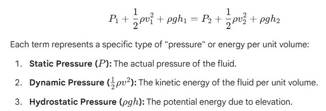
For any two points (1 and 2) along a pipe, the relationship is expressed as:

Each term represents a specific type of “pressure” or energy per unit volume:

1. Static Pressure (P): The actual pressure of the fluid.
2. Dynamic Pressure (1/2) *ρ v^2: The kinetic energy of the fluid per unit volume.
3. Hydrostatic Pressure (ρgh): The potential energy due to elevation.

The Relationship to Orifice Sizing

In orifice plate applications, we make two critical engineering assumptions to simplify the equation:

1. Horizontal Flow: The elevation change is negligible (h_1 = h_2), so the potential energy terms cancel out.
2. Energy Exchange: Since the total energy is constant, if the Velocity (v) increases due to a restriction, the Static Pressure (P) must decrease to compensate.

Real-World Engineering Deviations

Bernoulli’s “ideal” equation assumes no energy is lost. However, in practical instrumentation, we must account for “Real World” factors that Bernoulli ignored:

• Viscosity & Friction: Real fluids have internal friction, leading to a loss of energy as heat.
• Turbulence: The sudden contraction and expansion at the orifice plate create eddies and swirls.
• The Discharge Coefficient (C_d): This is the “fudge factor” engineers use to bridge the gap between Bernoulli’s theoretical flow and the actual flow measured in the field.
  • Theoretical Flow × C_d = Actual Flow
• The Trade-off: The “Differential Pressure” we measure (P_1 – P_2) is essentially the “Static Pressure” that was converted into “Kinetic Energy” to get the fluid through the hole.
• Density Sensitivity: Note that the fluid density (ρ) is a multiplier for the velocity term. This is why accurate density compensation (Pressure and Temperature correction) is vital for gas flow measurement—if your ρ is wrong in your flow computer, your Bernoulli-based calculation is fundamentally flawed.
• The Square Root Law: Because the velocity term (v) is squared in the equation, the resulting flow rate is proportional to the square root of the pressure drop ( √ΔP).

3: Governing Flow Equation (Full Form)

The ISO 5167 Mass Flow Formula

To calculate the actual mass flow rate (q_m), we modify the theoretical Bernoulli equation with empirical factors that account for real-world fluid dynamics.

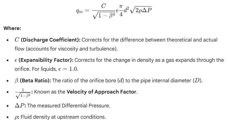
Key Assumptions & Boundary Conditions

For this equation to remain valid and maintain the stated uncertainty levels:

• Steady Flow: The flow must be single-phase and non-pulsating.
• Fully Developed Profile: The fluid must enter the orifice with a stable velocity profile (achieved via straight pipe runs).
• Subsonic Flow: The pressure drop must not reach critical (choked) flow conditions.
• Physical Integrity: The upstream edge of the plate must be sharp, and the plate must be flat.

Key Performance Indicators (KPIs) for the Equation

4: Key Sizing Variables

The accuracy of an orifice sizing calculation is only as good as the input data.

1. Mechanical Geometry

• Pipe Internal Diameter (D): Not the nominal size! You must use the actual ID based on the pipe schedule (e.g., Sch 40 vs. Sch 80). Even a 1mm deviation in D significantly shifts the β
• Orifice Bore Diameter (d): The calculated “hole” size. This is the value the vendor will machine to a high tolerance.
• Beta Ratio (beta = d/D): The dimensionless ratio that determines the “tightness” of the restriction.

2. Process & Fluid Dynamics

• Differential Pressure (Delta P): The “Full Scale” DP (e.g., 2500 mmH2O or 250 mbar). This determines the transmitter range.
• Density (ρ): Must be calculated at flowing conditions (operating P and T). For gases, this requires the Compressibility Factor (Z).
• Viscosity (mu): Directly impacts the Reynolds Number, which in turn dictates the Discharge Coefficient (C).

Engineering Checklist for Inputs

• Temperature & Pressure: Are these the “Normal” operating values or the “Maximum” design values? Sizing should typically be done for the maximum expected flow.
• Isentropic Exponent (kappa): For gas/steam, this is required to calculate the Expansibility Factor (ε).
• Pipe Roughness (k): Often overlooked, but internal corrosion or scaling changes the friction factor and flow profile.

Variable Sensitivity Analysis

 5: Beta Ratio Selection Criteria

The Beta Ratio (β = d/D) is the primary tuning knob in orifice design. While ISO 5167 provides a wide mathematical range, practical engineering usually dictates a much tighter window.

1. The Golden Range: 0.2 to 0.75

• ISO Limits: The standard validates the Discharge Coefficient (C) within these bounds.
• Engineering Sweet Spot: Most professionals aim for 3 to 0.6.
  • Below 0.2: The bore is so small that the pressure drop becomes excessive, and the risk of blockage or edge wear increases.
  • Above 0.75: The restriction is too “loose,” resulting in a weak Differential Pressure signal that is easily lost in process noise.

2. The Impact of β on Performance

• Low Beta (beta < 0.3): * Pros: High, stable Differential Pressure; excellent signal-to-noise ratio.
  • Cons: Extreme Permanent Pressure Loss (PPL); higher risk of plate deformation.
• High Beta (beta > 0.65): * Pros: Low pressure loss; energy efficient.
  • Cons: Weak signal; highly sensitive to upstream piping disturbances (requires longer straight runs).

3. The Engineering Trade-off

The selection process is a tug-of-war between two competing priorities:

1. Signal Strength: We want enough ΔP for the transmitter to read accurately (typically > 25 mbar).
2. Energy Recovery: We want to minimize the PPL to reduce pumping/compression costs.

Design Guidance Table

 6: Reynolds Number Considerations

The Reynolds Number (Re) is a dimensionless ratio of inertial forces to viscous forces. In orifice sizing, it tells us whether the fluid is moving in smooth layers or in a chaotic, tumbling fashion.

1. Definition and Calculation

For flow in a pipe, the Reynolds number is calculated as:

Re_D = ρ v D / μ

• ρ: Fluid density
• v: Velocity
• D: Pipe internal diameter
• μ: Dynamic viscosity

2. Flow Regimes

• Laminar (Re < 2000): Viscous forces dominate. The flow profile is parabolic. Orifice plates are not recommended here as the Discharge Coefficient (C_d) changes drastically with Re.
• Transitional (2000 < Re < 4000): The flow is unstable. Measurement is unpredictable and should be avoided.
• Turbulent (Re > 4000): Inertial forces dominate. The velocity profile is flatter, and the Discharge Coefficient becomes much more stable (predictable).

3. ISO 5167 Validity Limits

To maintain the uncertainty levels defined in the standard, ISO 5167 imposes a Lower Limit for Re.

• Typically, for a standard concentric orifice, Re_D must be > 5000.
• If your process operates below this limit (e.g., highly viscous oils), the standard C_d equations no longer apply, and you must use a Quadrant Edge or Conical Entrance orifice plate.

Engineering Impact Table

 7: Discharge Coefficient (C_d)

The Discharge Coefficient is the ratio of the actual mass flow to the theoretical mass flow. It accounts for the contraction of the flow stream (Vena Contracta) and energy losses due to friction.

1. The Empirical Correlation

Unlike basic physics constants, C_d is derived from thousands of flow lab tests. It is not a single number but a variable that depends on:

• The Beta Ratio (β): How much the flow is constricted.
• The Reynolds Number (Re): How turbulent the flow is.
• Tapping Locations: Whether you are using Flange, Corner, or D and D/2 taps.

2. The ISO 5167 Polynomial (Reader-Harris/Gallagher Equation)

Modern sizing uses the RG equation, a complex polynomial adopted by ISO 5167.

• It eliminates the need for manual look-up charts.
• It ensures that the C_d stays predictable across a wide range of pipe sizes and flow conditions.
• The equation includes terms for the “velocity of approach” and the specific geometry of the tapping points.

3. The “Sharp Edge” Requirement

The math assumes an infinitely sharp upstream edge.

• Edge Sharpness: The radius of the upstream edge must be less than 0004d.
• Plate Wear/Dulling: As the edge rounds off due to erosion or corrosion, the C_d This leads to “Under-reading” the transmitter sees less ΔP than it should for a given flow, causing the flow computer to report a lower flow rate than what is actually passing through.

Maintenance Impact on C_d

 8: Expansibility Factor (ε) for Gas/Steam

When a liquid passes through an orifice, its density remains constant. However, when a gas or steam passes through, the pressure drop at the bore causes the fluid to expand, changing its density instantaneously. The Expansibility Factor (ε) is the correction for this phenomenon.

1. Compressible Flow Correction

If we used the standard flow equation for gas without ε, we would significantly over-estimate the mass flow. The factor ε accounts for the adiabatic expansion of the gas as it moves from the upstream tapping to the vena contracta.

• For Liquids: ε = 1.0 (incompressible).
• For Gases/Steam: ε < 1.0 (typically between 95 and 0.99).

2. The Mathematical Dependencies

The value of ε is not a constant; it is a dynamic variable calculated based on:

• Pressure Ratio (Delta P / P_1): The ratio of the differential pressure to the absolute upstream pressure.
• Isentropic Exponent (kappa): Also known as the ratio of specific heats (C_p/C_v), which varies by gas composition.
• Beta Ratio (β): The physical geometry of the restriction.

3. Importance in High-Pressure Systems

In high-pressure gas systems (e.g., natural gas transmission), a small error in ε calculation leads to massive financial discrepancies.

• The 25% Rule: To keep uncertainty low, ISO 5167 generally recommends that the ratio ΔP / P_1 should be less than 25. If the pressure drop is too high relative to the line pressure, the expansion becomes too violent to model accurately with standard empirical formulas.

Sensitivity Check: Ε Impact

9: Fluid Property Inputs (Critical for Accuracy)

The orifice plate formula is a “Snapshot in Time.” If the fluid properties at the moment of measurement don’t match the design data, the resulting flow rate is a fiction.

1. Density at Flowing Conditions (ρ_f)

This is the single most influential fluid property.

• Liquid Service: Density varies primarily with Temperature. Thermal expansion can change density by 1% to 1% per 10^°C.
• Gas Service: Density is a slave to both Pressure and Temperature (PV=nRT).
• The Rule: Always use density at the upstream tapping point pressure and temperature.

2. Viscosity and Temperature Dependence (μ)

While density affects the “weight” of the flow, viscosity affects the “friction.”

• As temperature increases, liquid viscosity usually decreases, while gas viscosity increases.
• Impact: Viscosity defines the Reynolds Number. If viscosity is incorrectly modeled, the flow computer selects the wrong Discharge Coefficient (C_d).

3. Compressibility Factor (Z)

For “Real” gases (as opposed to Ideal gases), the Z factor accounts for the deviation from the Ideal Gas Law.

• At high pressures, gas molecules are forced so close together that their own volume and intermolecular forces matter.
• Z ≠ 1.0: Failing to account for Z in high-pressure natural gas or hydrogen can result in errors exceeding 5%.

4. Phase Behavior

• Single Phase: The orifice math assumes 100% liquid or 100%
• The Multiphase Trap: If a liquid “flashes” into a gas at the orifice due to the pressure drop, or if a gas contains “slugs” of liquid (wet gas), the standard ISO 5167 equations are invalid. This leads to massive over-reading or under-reading.

Impact of Property Deviations

 10: Differential Pressure Selection Philosophy

Selecting the maximum Differential Pressure (ΔP_max) is not a random choice; it is a strategic decision that dictates the sensitivity, accuracy, and energy footprint of the measurement loop.

1. Typical Engineering Ranges

While technology allows for extreme ranges, industry standard practice generally falls into these buckets:

• Low DP (5–50 mbar): Used for low-pressure gas ducts or large diameter pipes where pressure loss must be near zero.
• Standard DP (50–500 mbar): The “sweet spot” for most oil, gas, and water applications.
• High DP (>500 mbar / up to 1000 kPa): Used in high-pressure systems where the static pressure is high enough to “mask” the pressure loss, or where a small bore is required for high-velocity fluids.

2. Turndown and Signal-to-Noise Ratio

• The Square Root Constraint: Because Flow α √ΔP, a 10:1 turndown in flow requires a 100:1 turndown in ΔP.
• Signal-to-Noise: If you select a ΔP_{max} that is too low, the signal at low flow rates becomes indistinguishable from process “noise” (turbulence, vibration), leading to an unstable reading.
• Transmitter Capability: Modern “Smart” transmitters can handle high turndown, but the primary element (the plate) still limits the physical accuracy at the low end.

3. Application-Specific Criteria

• Control Loops: Reliability and speed are key. Moderate ΔP is preferred to ensure a clean signal for the PID controller.
• Monitoring/Measurement: Balanced approach focusing on low PPL and reasonable accuracy.
• Custody Transfer: High ΔP is often preferred to maximize resolution and accuracy, provided the pressure loss is acceptable to the stakeholders.

DP Selection Guide

 11: Permanent Pressure Loss (PPL)

The differential pressure (ΔP) we measure at the taps is not the final cost to the process. While some pressure is recovered downstream, a significant portion is lost forever due to friction and turbulence.

1. The Relationship with β and ΔP

The amount of pressure lost is directly tied to the Beta ratio. The smaller the hole (lower β), the more energy is converted into heat and noise rather than being recovered.

• Approximate Formula: The PPL can be estimated as:

• Visualizing the Loss: As β increases, the “obstruction” becomes less severe, allowing for better pressure recovery.

2. Typical PPL Ranges

In standard orifice installations, you should expect to lose a massive chunk of your measured signal:

• Typical Loss: 40% to 70% of the measured ΔP.
• Example: If you measure a ΔP of 250 mbar and your β is 0.5, your permanent loss will be approximately 180 mbar.

3. Energy Cost Implications

Pressure loss is not “free.” It must be compensated for by pumps (for liquids) or compressors (for gases).

• OPEX Impact: Over a 10-year period, the electricity cost to overcome the PPL of a single orifice plate in a large-diameter high-pressure line can exceed the initial cost of an Ultrasonic or Coriolis meter.
• Carbon Footprint: In modern “Green” engineering, high PPL is increasingly scrutinized as a source of unnecessary CO_2 emissions due to wasted pump/compressor energy.

PPL Comparison Table

12: Straight Run Requirements

The mathematical validity of the ISO 5167 equations depends entirely on a fully developed, symmetrical flow profile. If the fluid is swirling or “jetting” to one side, the Discharge Coefficient (C_d) becomes meaningless.

1. Upstream and Downstream Mandates

• Upstream: Generally requires 10D to 44D (diameters) of straight pipe, depending on the Beta ratio and the type of upstream disturbance.
• Downstream: Generally requires 2D to 8D to allow for pressure recovery and to ensure the downstream tapping isn’t influenced by a downstream fitting.
• The Beta Factor: As the Beta ratio (β) increases, the required straight run increases significantly because a larger bore is more sensitive to profile distortions.

2. Common Disturbance Effects

• Single Elbows: Create a skewed velocity profile.
• Two Elbows (Out-of-Plane): These are the most dangerous; they generate Swirl, which can persist for over 50 diameters and cause massive measurement errors.
• Valves/Tees: Create severe turbulence. Control valves should always be located downstream of the orifice if possible.

3. Flow Conditioners: The “Short-Cut”

When the physical plant layout doesn’t allow for long straight runs, we use flow conditioners to “force” the flow into a developed state.

• Tube Bundles: Good for straightening flow but ineffective against swirl.
• High-Performance Conditioners (Zanker, Laws, Gallagher): Perforated plates that remove swirl and redistribute the velocity profile in as little as 6D to 8D.

Piping Configuration Impact

 14: Tappings Configurations

The tapping configuration defines the distance from the orifice plate to the pressure sensing points. Each configuration has a specific “coefficient footprint” and preferred industrial application.

1. Common Industrial Configurations

• Flange Taps: The most popular in the Oil & Gas industry. Taps are located exactly 1 inch (25.4 mm) upstream and downstream from the plate faces. They are integrated into the orifice flange union, making them easy to manufacture and inspect.
• Corner Taps: Taps are located at the “corners” where the plate meets the pipe wall. Commonly used for smaller pipe sizes (D < 50 mm) or in European DIN standards. They are excellent for measuring “clean” fluids.
• D and D/2 Taps (Radius Taps): The upstream tap is at 1D and the downstream tap is at 5D from the plate. This is theoretically superior because the downstream tap sits right near the Vena Contracta (the point of lowest pressure).
• Pipe Taps (2.5D and 8D): Taps are located far upstream and far downstream. These measure the “Permanent Pressure Loss” rather than the maximum ΔP. They are rarely used in modern precision measurement.

2. Impact on the Discharge Coefficient (C_d)

• The Pressure Gradient: Because the pressure changes rapidly as the fluid approaches and exits the orifice, moving the tap even a few millimeters changes the measured ΔP.
• Standard Compliance: ISO 5167 provides different coefficients for each tap type. If your transmitter is connected to Flange Taps but your flow computer is programmed for Corner Taps, your flow reading will be fundamentally incorrect.

Configuration Comparison Table

 15: Plate Types and Geometry

While the concentric, sharp-edged plate is the default, certain process conditions—such as entrained solids, gas bubbles in liquids, or high viscosity—require specialized geometries to prevent measurement failure.

1. Concentric Sharp-Edged (The Standard)

• Design: The hole is centered in the pipe.
• Use Case: Ideal for clean liquids, gases, and steam.
• Constraint: Prone to debris buildup (damming) at the bottom of the pipe for liquids or liquid trapping for gases.

2. Eccentric Orifice

• Design: The bore is shifted so it is nearly flush with the bottom (for solids) or top (for gases) of the pipe.
• Use Case: Measuring liquids containing small amounts of solids/sludge or gases containing some liquid condensate.
• Benefit: Prevents the “damming” effect, allowing secondary phases to pass through without affecting the ΔP.

3. Segmental Orifice

• Design: The “bore” is a semi-circle or segment of a circle, usually at the bottom of the pipe.
• Use Case: Heavy slurries, extremely dirty fluids, or sewage.
• Benefit: Provides an almost completely unobstructed path at the bottom of the pipe for heavy particles.

4. Quadrant Edge Orifice

• Design: The upstream edge is not sharp but rounded (a quarter-circle).
• Use Case: High viscosity fluids (low Reynolds Number, Re < 10,000).
• Benefit: Unlike sharp edges, where C_d changes wildly at low Re, the rounded edge provides a constant Discharge Coefficient in the laminar/transitional transition zone.

Selection Matrix: Which Plate to Use?

 16: Orifice Plate Materials

The orifice plate is a “sacrificial” element exposed to the highest velocity and turbulence in the pipe. Its material must be selected to resist chemical attack, physical erosion, and mechanical deformation.

1. Common Metallurgies

• SS316/316L: The industry baseline. Excellent for general water, air, and “sweet” (low H_2S) hydrocarbons.
• Monel 400: Preferred for hydrofluoric acid or oxygen service.
• Inconel / Incoloy: Used for extreme high-temperature applications or highly corrosive environments.
• Duplex / Super Duplex: Offers superior mechanical strength and resistance to chloride stress corrosion cracking.
• Hastelloy C276: The “universal” solution for aggressive chemical services and highly corrosive “sour” gas.

2. NACE Compliance & Hardness

• NACE MR0175 / ISO 15156: Critical for upstream oil and gas. Materials must be resistant to Sulfide Stress Cracking (SSC).
• Hardness Limits: To meet NACE standards, materials like SS316 must typically have a hardness below 22 HRC (Rockwell C).
• The Conflict: High hardness is good for resisting erosion but bad for resisting stress corrosion in sour service.

3. Corrosion, Erosion, and Wear

• Erosion: High-velocity particles (sand/scale) can round the sharp upstream edge. Even a few microns of wear can lead to a 2–5% measurement error.
• Corrosion: Pitting on the plate surface increases pipe roughness, which disrupts the velocity profile.
• Stellite Facing: For extremely abrasive flows, the upstream edge can be “hard-faced” with Stellite to maintain sharpness for a longer duration.

Material Selection Quick-Reference

 17: Plate Thickness and Flatness Criteria

The mechanical integrity of the plate ensures it does not vibrate or deform under high Differential Pressure (ΔP). Even a slight “bow” in the plate can lead to significant measurement bias.

1. ISO 5167 Thickness Guidelines

The standard defines two critical thickness dimensions:

• Plate Thickness (E): The overall thickness of the metal disc. It must be sufficient to prevent the plate from bending or “dishing” under the force of the flow.
• Bore Edge Thickness (e): The thickness of the cylindrical part of the bore. This must be much thinner than the plate itself (typically between 005D and 0.02D).
• The Rule: If the plate is too thick at the bore, it starts to act like a short tube rather than an orifice, which changes the Discharge Coefficient (C_d).

2. Flatness Tolerance

• The Requirement: The plate must be flat to within 1% of the pipe radius (01 \times D/2) across its entire surface.
• The “Dishing” Effect: Under high pressure, plates can warp. If a plate is not flat, the flow lines do not strike it at a 90-degree angle, causing the Vena Contracta to shift and the meter to under-read.

3. Upstream Edge & Bevel Angle

• Edge Sharpness: As discussed, the upstream edge must not reflect light when viewed without magnification. It must be a perfect 90-degree corner.
• The Bevel: Because the plate thickness (E) is usually greater than the required edge thickness (e), the downstream side must be beveled at an angle between 30^\circ and 45^\circ. This ensures the fluid only “sees” the sharp upstream edge.

Physical Criteria Summary

 18: Bore Measurement and Tolerance

The orifice bore diameter (d) is the primary geometric variable in the flow equation. Because the flow rate is proportional to the square of the bore diameter (d^2), even a microscopic error in measurement leads to a significant error in the reported flow.

1. Bore Measurement Techniques

To achieve the required precision, measurements must be taken at multiple points using calibrated instruments:

• Internal Micrometers / Bore Gauges: Used to take measurements at at least four equally spaced diameters (every 45°).
• CMM (Coordinate Measuring Machine): Used in high-precision labs to map the circularity and concentricity of the bore.
• Thermal Compensation: Large plates should be measured at a controlled temperature (typically 20°C) to account for thermal expansion/contraction of the metal.

2. Tolerance Requirements

ISO 5167 and ASME MFC-3M mandate strict tolerances for the bore:

• Typical Tolerance: ±0.01 mm to ±0.05 mm depending on the pipe size.
• Circularity: The difference between any two measured diameters must be less than 05% of the mean bore diameter.
• Edge Sharpness: As discussed previously, the upstream edge must be sharp enough to not reflect a beam of light.

3. Impact on Flow Uncertainty

The mathematical impact of a bore measurement error is amplified by the “Power of 2.”

• The Math: A 5% error in measuring the bore diameter results in approximately a 1.0% error in the calculated mass flow.
• Cumulative Risk: If you combine a poor bore measurement with a poor pipe ID measurement, your Beta (β) ratio uncertainty becomes the dominant source of error in your entire flow loop.

Sensitivity Analysis: Bore Error

 19: Installation Effects on Accuracy

Even a perfectly sized and machined orifice plate will fail to meet its uncertainty targets if it is not installed with surgical precision. Installation errors are “silent killers” of accuracy because they often leave no external signs of failure.

1. Misalignment and Eccentricity

The orifice bore must be perfectly concentric with the pipe centerline.

• The Error: If the plate is “dropped” or shifted to one side during installation, the flow profile becomes asymmetric.
• Impact: Eccentricity causes the fluid to “bunch up” on one side of the bore, leading to a shift in the Discharge Coefficient (C_d). This can introduce errors of 1% to 5% depending on the severity and the Beta ratio.

2. Plate Orientation Errors (The “Backwards” Plate)

One of the most common—and embarrassing—field errors is installing the plate backward.

• The Physics: The sharp edge must face upstream. The bevel must face downstream.
• The Result: If the bevel faces the flow, the fluid “glides” through the restriction rather than separating cleanly. This results in a massive under-reading (up to 15–20%) of the actual flow rate.

3. Gasket Intrusion and Bolt Torque

• Gasket Protrusion: If a gasket is too small or improperly centered, it can protrude into the pipe ID. This creates an unplanned disturbance right before the plate, destroying the velocity profile.
• Uneven Bolt Torque: Excessive or uneven tightening can “bow” the orifice flanges or the plate itself, especially in high-pressure applications. As we discussed, a non-flat plate is a non-accurate plate.

Installation Troubleshooting Checklist

 20: DP Transmitter Selection

The Differential Pressure (DP) transmitter is responsible for converting the physical pressure drop into a digital or 4-20mA signal. Choosing the wrong transmitter can negate all the precision engineering put into the orifice plate.

1. Range Selection and Turndown

• URL vs. Span: The Upper Range Limit (URL) is the maximum the sensor can physically measure. The Span is the specific range you calibrate for (e.g., 0–250 mbar).
• Turndown Reality: While modern “Smart” transmitters claim 100:1 or even 200:1 turndown, the uncertainty increases at the bottom of the range. For orifice measurement, a practical turndown of 5:1 or 10:1 is typical to maintain ±1% accuracy.
• Square Root Extraction: Most modern transmitters can perform the square root extraction internally, providing a linear flow signal to the DCS/PLC.

2. Static Pressure Rating

• The “Zero Shift” Effect: DP transmitters are often used in high-pressure lines (e.g., 100 bar) to measure a tiny pressure drop (e.g., 250 mbar).
• Line Pressure Influence: High static pressure can cause the sensor to “shift” its zero point. High-quality transmitters include internal sensors to compensate for this static pressure effect in real-time.

3. Remote Seals vs. Impulse Lines

• Impulse Lines: Standard for clean gases and liquids. Uses small-bore tubing to bring the pressure to the transmitter.
• Remote Seals (Capillaries): Used for corrosive, viscous, or hygienic fluids where the process must not enter the transmitter body.
  • Warning: Capillaries are sensitive to ambient temperature changes, which can cause measurement “drift.”

4. Smart Transmitter Diagnostics

Modern “Smart” (HART/Foundation Fieldbus) transmitters offer more than just a PV:

• Plugged Impulse Line Detection: Analyzes the “noise” spectrum of the process to detect if a sensing line is blocked.
• Loop Integrity: Monitors for power supply issues or high-impedance connections.
• Sensor Health: Tracks over-pressure events that might have damaged the diaphragms.

Transmitter Selection Checklist

 21: Impulse Line Design

The impulse lines are the small-bore pipes or tubes that transmit the pressure signal from the orifice tappings to the DP transmitter. Their design must ensure that the pressure reaches the sensor without distortion, lag, or blockage.

1. Service-Specific Orientation

The physical orientation of the transmitter relative to the pipe depends entirely on the fluid phase:

• Gas Service: The transmitter should be mounted above the orifice. Impulse lines should slope upward so any liquid condensate drains back into the process pipe.
• Liquid Service: The transmitter should be mounted below the orifice. Impulse lines should slope downward so any trapped gas bubbles can rise back into the process pipe.
• Steam Service: Mounted below the orifice (similar to liquid) to ensure the impulse lines remain filled with water (condensate) to protect the transmitter from high temperatures.

2. Condensate Pots for Steam

• Purpose: In steam measurement, we cannot allow live steam to touch the transmitter diaphragms.
• Function: Condensate pots provide a reservoir of water at a constant level. This ensures that the “head” of liquid on both the high and low-pressure sides remains equal, preventing a false differential pressure reading.

3. Slope and Blockage Prevention

• Minimum Slope: A slope of at least 1:12 (8%) is recommended to ensure the natural migration of bubbles or condensate.
• Support: Lines must be properly supported to prevent “sags” where liquid (in gas lines) or gas (in liquid lines) can become trapped, creating a “vapor lock.”
• Manifolds: A 3-way or 5-way valve manifold is essential for zeroing the transmitter, bleeding air, and isolating the instrument for maintenance.

Impulse Line Design Summary

 22: Temperature Measurement Integration

Temperature is not just a process variable; it is a mathematical requirement for flow calculation. Because density is a function of temperature, an error in temperature measurement translates directly into a flow measurement error.

1. Importance of RTD/Thermowell Location

To get an accurate “flowing temperature,” the sensor must be close enough to the orifice to be representative, but far enough away to avoid disturbing the flow profile.

• Downstream is Best: Standard practice (ISO 5167) recommends placing the thermowell downstream of the orifice plate.
• Distance: Typically 5D to 15D If placed upstream, it must be significantly further away (up to 44D) to ensure the wake from the thermowell doesn’t hit the orifice plate.
• Immersion Depth: The RTD tip must reach the center third of the pipe to avoid “wall effects” where the pipe metal temperature influences the reading.

2. Density Compensation in Flow Computers

Modern flow computers use the live temperature (T) and pressure (P) inputs to solve the state equations in real-time.

• The Sensitivity: In natural gas, a 3^°C error in temperature measurement can result in a 5% to 1% error in mass flow.
• Linear vs. Real: While some systems use a simple linear thermal expansion coefficient for liquids, high-pressure gas systems require complex models (like AGA8) to account for how temperature affects the compressibility factor (Z).

3. Lag and Response Time Effects

• Thermal Mass: Heavy-duty thermowells act as a “heat sink,” causing a delay (lag) between a change in fluid temperature and the RTD’s response.
• Dynamic Errors: During rapid process swings (e.g., startup or batching), the flow computer might use an “old” temperature reading with a “new” pressure reading, leading to temporary but significant flow spikes or dips.
• Solution: Use high-response RTDs and thermowells with thermal paste to minimize the air gap and improve heat transfer.

Temperature Impact Analysis

 24: Uncertainty Analysis

No measurement is perfect. Uncertainty analysis is the statistical method used to quantify the “doubt” in a measurement result. In orifice systems, the total uncertainty is the root-sum-square of the uncertainties of every individual component.

1. Sources of Error (The “Uncertainty Budget”)

The total uncertainty in mass flow (U_{qm}) is influenced by both the primary element and the secondary instrumentation:

• Primary Element (C_d): The ISO 5167 Discharge Coefficient typically carries an inherent uncertainty of ± 0.5% to 0.6%.
• Differential Pressure (ΔP): Includes transmitter accuracy, drift, and static pressure effects.
• Fluid Density (ρ): Derived from the uncertainties in pressure and temperature measurements and the Equation of State (Z-factor).
• Geometry (D and d): Uncertainties in the measured pipe ID and the orifice bore.

2. Combined Uncertainty Calculation

According to the law of propagation of uncertainty, the individual components are combined as follows (simplified):

Note: Because flow is a square root function, the uncertainty of ΔP and density are halved in their contribution to the total.

3. Typical Overall Accuracy

• Standard Industrial: ± 1.0% to 2.0% of actual flow.
• Optimized / Custody Transfer: ± 0.5% to 1.0% (requires high-precision bore measurement, calibrated transmitters, and live P&T compensation).
• Degraded Systems: > 5% (caused by poor straight runs, dull plate edges, or uncompensated gas flow).

Uncertainty Component Impact

 25: Sizing for Control vs. Measurement

The design objectives for an orifice plate change depending on whether the signal is used for accounting (Measurement) or for a PID control loop (Control).

1. Control Valve Interaction with DP

When an orifice is placed in series with a control valve, they compete for the available pressure drop in the line.

• The Conflict: To save energy, we want a low ΔP across the orifice. However, a control valve requires a certain “pressure drop ratio” to maintain control over the flow.
• Pressure Drop Ratio: If the orifice ΔP is too high relative to the valve’s ΔP, the valve loses its ability to influence flow effectively until it is nearly closed.

2. Signal Linearization Issues

Because of the Square Root Relationship (Q \propto \sqrt{ΔP}), the sensitivity of the measurement changes across the range.

• Low Flow Sensitivity: At the bottom 10% of flow, the ΔP is only 1% of the full scale. Small process “noise” or transmitter drift can cause the PID controller to perceive massive flow swings that aren’t actually happening.
• Loop Gain: The “gain” of the flow measurement is non-linear. This makes PID tuning difficult unless the signal is linearized (square root extraction) before it reaches the controller.

3. Valve Authority and Loop Stability

• Valve Authority: This is the ratio of the pressure drop across the valve at full flow to the total system pressure drop. A poorly sized orifice can “rob” the valve of its authority.
• Steady Signal: For control, a stable signal is often more important than an accurate A slightly higher β (Beta ratio) might be chosen to reduce turbulence and signal “jitter,” providing a smoother input for the PID algorithm.

Design Priority Comparison

 26: Multiphase and Wet Gas Issues

Standard orifice plate correlations (ISO 5167) are strictly designed for single-phase fluids. When gas contains liquid droplets (Wet Gas) or liquid contains gas bubbles, the physics of the pressure drop changes fundamentally.

1. Slip and Phase Distribution

• The Slip Phenomenon: In a multiphase stream, the gas and liquid phases do not travel at the same velocity. The gas, being less dense, “slips” past the liquid.
• Flow Regimes: Depending on the velocity, the liquid might travel as a film along the pipe wall (annular flow), in slugs, or as a fine mist. Each regime affects the orifice plate differently.

2. Over-reading and Under-reading Errors

• The “Over-reading” Effect: In wet gas measurement, the orifice plate almost always over-reads the gas flow rate. Because the plate is “fooled” by the extra momentum of the liquid droplets, it produces a higher ΔP than the gas would alone.
• Magnitude of Error: Without correction, a liquid volume fraction of just 5% can lead to a gas flow measurement error of 20% to 30%.

3. Correction Models (The Solutions)

Since a standard calculation fails, engineers use specialized empirical models to “back out” the true gas flow:

• Lockhart-Martinelli Parameter (\chi): A dimensionless number used to characterize the “wetness” of the gas.
• Murdock & Chisholm Correlations: Classic equations that apply a correction factor to the gas flow based on the estimated amount of liquid.
• Dual DP Measurement: Using two different primary elements (e.g., an orifice and a Venturi) in series to solve for both the gas and liquid flow rates simultaneously.

Multiphase Impact Summary

 27: High-Pressure Gas Orifice Design

In high-pressure gas applications (e.g., gas injection, transmission, or relief systems), the fluid energy is immense. Design must account for the transition from subsonic to sonic flow and the physical forces acting on the plate.

1. Choked Flow and Critical Pressure Ratio

• The Phenomenon: As the pressure drop (ΔP) across the orifice increases, the velocity at the bore increases. Eventually, the velocity reaches the Speed of Sound (Mach 1).
• The Limit: Once the flow is “choked,” increasing the downstream pressure drop further will not increase the mass flow rate.
• Critical Pressure Ratio (r_c): This is the ratio of downstream to upstream pressure (P_2/P_1) where choking occurs. For natural gas, this is typically around 54.
  • Sizing Rule: To use ISO 5167 measurement equations, you must stay well away from this ratio (typically ΔP/P_1 < 0.25).

2. Sonic Velocity Limitations

• Noise and Vibration: Approaching sonic velocity creates intense acoustic energy. This can lead to acoustic fatigue in the piping.
• Standard Deviation: The Expansibility Factor (\ε) we discussed in 9 becomes highly non-linear near sonic speeds. Standard orifice sizing software will usually throw a warning if the “Mach Number” at the bore exceeds 3 to 0.4.

3. Plate Stress and Mechanical Integrity

High-pressure gas creates a massive physical load on the orifice plate (the “Piston Effect”).

• Bending Stress: The plate must be thick enough to resist the total force (F = ΔP \times Area). If the plate bows, the measurement is ruined; if it yields, it can be sucked into the downstream pipe.
• Buckling: In high-pressure transients (e.g., sudden valve opening), the impact of the gas “slug” can cause the plate to buckle or dislodge from the carrier.
• Sizing Check: Always verify the Maximum Differential Pressure (Static) that the plate can withstand without permanent deformation.

High-Pressure Design Constraints

 28: Steam Flow Orifice Design

Steam measurement requires a multidisciplinary approach combining fluid dynamics with thermodynamics. Because steam density is highly sensitive to pressure and temperature, the “State” of the steam—Saturated or Superheated—dictates the sizing logic.

1. Saturated vs. Superheated Corrections

• Saturated Steam: In this state, pressure and temperature are linked. If you know the pressure, the temperature is fixed (and vice versa).
  • The Risk: If the steam loses heat, it becomes “Wet Steam” (quality < 100%). The presence of water droplets causes the orifice to over-read, similar to the wet gas effect.
• Superheated Steam: Functions more like a “Real Gas.” Pressure and temperature are independent variables.
  • The Requirement: You must measure both P and T Compensation must account for the specific enthalpy and density changes using IAPWS-IF97 standards.

2. Condensate Management

Steam is a gas that lives at its boiling point. Any cooling in the impulse lines will turn the steam into water.

• The Head Error: If the water level in the high-pressure (HP) impulse line is different from the low-pressure (LP) line, it creates a “false DP.”
• The Solution: Use Condensate Pots (also called Seal Pots). These act as reservoirs that maintain a constant, equalized liquid head on both sides of the transmitter, protecting the sensor from the 200^°C+ temperatures while ensuring a stable signal.

3. ISO Steam Tables Integration

To achieve high accuracy, the flow computer must use the IAPWS-IF97 (International Association for the Properties of Water and Steam) correlations.

• Real-time Calculation: The computer continuously calculates the Isentropic Exponent (k) and Density (ρ).
• The Error of Simplicity: Using a fixed density for steam is never recommended; a 5% change in steam pressure can lead to a nearly 5% error in mass flow if not dynamically compensated.

Steam Design Comparison

 29: Liquid Flow Orifice Design

When sizing for liquids, the “speed bump” created by the orifice plate can cause the local pressure to drop below the fluid’s vapor pressure. This leads to two destructive phenomena: Flashing and Cavitation.

1. Cavitation and Flashing Risk

• The Vena Contracta Effect: The lowest pressure occurs just downstream of the orifice bore.
• Cavitation: If the pressure drops below the vapor pressure at the bore but recovers above it further downstream, bubbles form and then violently collapse. This collapse sends shockwaves that can pit and “eat” the stainless steel plate and pipe wall.
• Flashing: If the downstream pressure never recovers above the vapor pressure, the liquid stays as a vapor. This creates “choked flow” for liquids, making the standard \sqrt{ΔP} math completely invalid.

2. Minimum Pressure Drop Constraints

While we often worry about having too much pressure drop, having too little is also a risk for liquids:

• Signal Strength: If the ΔP is too low (below 10–25 mbar), the transmitter cannot distinguish between actual flow and the “head” of the liquid in the impulse lines.
• The Sizing Rule: Always ensure the operating ΔP is at least 10 times the expected uncertainty of the transmitter’s zero-point.

3. Noise and Vibration Considerations

• Turbulence: High-velocity liquid hitting a sharp restriction creates mechanical vibration. If the frequency of this vibration matches the natural frequency of the orifice plate, the plate can suffer fatigue failure.
• Acoustic Noise: While less common than in gas, high-velocity liquid flow (especially during cavitation) can produce noise levels exceeding 85 dBA, requiring acoustic insulation or a change in plate design (e.g., a multi-hole plate).

Liquid Design Guardrails

 30: Noise and Vibration in Orifice Systems

An orifice plate is a flow obstruction that converts pressure energy into kinetic energy and, inevitably, into acoustic and mechanical energy. In high-pressure or high-velocity systems, this can lead to severe noise pollution and “Flow-Induced Vibration” (FIV).

1. Turbulence-Induced Vibration

• Vortex Shedding: As fluid passes the sharp edge of the plate, it creates a trail of turbulent eddies (Von Kármán vortices).
• Mechanical Fatigue: If the frequency of these vortices matches the natural frequency of the orifice plate or the surrounding pipework, resonance occurs. This can lead to “fatigue cracking” at the orifice flange or impulse line connections.
• The “Singing” Orifice: High-frequency vibration often manifests as a distinct whistle or hum.

2. Acoustic Noise Prediction

• The Source: Noise is primarily generated by the rapid expansion of gas or the collapse of cavitation bubbles in liquids.
• Variables: Noise levels (dBA) increase with the Mass Flow Rate, the Pressure Ratio, and the Beta Ratio.
• Standard Limits: Most plants mandate noise levels below 85 dBA at one meter. Exceeding this requires either heavy-duty pipe insulation or a design change.

3. Mitigation Strategies

• Multi-Hole Plates (Conditioning Orifices): Instead of one large bore, the plate has many smaller holes. This breaks up large turbulent structures into smaller, higher-frequency eddies that dissipate more quickly and quietly.
• Diffuser Plates: A second perforated plate installed downstream can help stage the pressure drop, preventing the “shock” of a single large expansion.
• Downstream Back-Pressure: In liquid systems, ensuring sufficient downstream pressure can “smother” cavitation before it begins.
• Heavy-Wall Piping: Increasing the pipe schedule (e.g., from Sch 40 to Sch 80) can provide better acoustic dampening.

Noise & Vibration Troubleshooting

 31: Multi-Hole and Conditioning Orifice Plates

Traditional single-bore orifice plates are limited by their sensitivity to flow profiles and their narrow accurate range. Conditioning Orifice Plates utilize a multi-hole pattern to “self-condition” the flow as it passes through the element.

1. Flow Conditioning Plates

• The Design: Instead of one central hole, these plates typically feature four or more symmetrical bores.
• The “Zero-Straight-Run” Advantage: Because the flow is split into multiple streams, the plate effectively “re-profiles” the velocity distribution. This allows for accurate measurement with as little as 2D upstream and 2D downstream straight runs.
• Eliminating Swirl: The multi-hole geometry acts as a physical baffle that kills the swirl generated by out-of-plane elbows or valves.

2. High Turndown Ratio Applications

• Stable ΔP: In a standard orifice, the “dead zone” at low flow is a major limitation. Multi-hole plates produce a more stable and “quiet” ΔP
• Extended Range: Because the signal-to-noise ratio is improved, many conditioning plates can achieve a turndown of 10:1 or 14:1, compared to the typical 3:1 or 4:1 of a standard concentric plate.
• Low-Flow Accuracy: Better pressure recovery and reduced turbulence at the taps allow for more reliable readings at the bottom end of the transmitter’s range.

3. Compact Installations (Skid and Offshore)

• Space & Weight Savings: In offshore platforms or modular chemical skids, space is expensive. Eliminating 20 meters of straight piping by using a conditioning plate can save thousands in structural steel and piping costs.
• Integrated Manifolds: These plates are often sold as “Compact Orifice” units, where the plate, manifold, and transmitter are pre-assembled as a single, “wafer-style” component.

Standard vs. Conditioning Orifice

 32: Special Applications

When a fluid is extremely cold, abrasive, or thick, a standard SS316 concentric plate will fail. These special applications require unique metallurgy, geometry, and installation techniques.

1. Cryogenic Fluids (LNG, Liquid Nitrogen/Oxygen)

• The Thermal Expansion Challenge: Metals shrink significantly at cryogenic temperatures (e.g., -162 °C for LNG).
  • The Fix: Sizing software must use the Linear Coefficient of Thermal Expansion to calculate the “Actual” bore diameter at operating temperature. If you measure the bore at 20^\circC but operate at -160 °C, your d will be smaller than expected, leading to a massive over-reading.
• Material Integrity: Standard carbon steel is brittle at these temperatures. SS304/316 or specialized alloys are required to maintain impact strength.
• Boiling Risk: Cryogenic fluids are often close to their boiling point; the ΔP across the orifice must be kept very low to prevent flashing in the line.

2. Corrosive and Erosive Slurries

• Slurry Dynamics: Solid particles in a carrier liquid will settle and “dam” behind a standard plate.
• The Segmental Solution: Use a Segmental Orifice (where the bore is a semi-circle at the bottom of the pipe). This allows solids and rocks to pass through while the top segment measures the flow.
• Hardfacing: For erosive slurries (sand/mining), the upstream edge is often coated with Stellite or Tungsten Carbide to prevent the “rounding” of the edge that causes measurement drift.

3. High-Viscosity and Low-Re Flows

• The Viscosity Trap: As discussed in 7, when Re < 5,000, the Discharge Coefficient (C_d) of a sharp-edged plate becomes unstable.
• The Conical Entrance / Quadrant Edge: * Conical Entrance: Features a 45° bevel on the upstream
  • Quadrant Edge: Features a rounded, quarter-circle upstream profile.
• Benefit: These shapes “guide” the viscous fluid through the restriction, keeping the C_d relatively constant even when the fluid is thick (e.g., heavy fuel oil, bitumen, or polymers).

Application Selection Guide

33: Orifice Sizing Workflow (Engineering Steps)

Sizing an orifice is an iterative process. You rarely get the perfect “Beta” on the first try. Following a structured workflow ensures that the final design is both accurate and safe for the process.

1. Define Process Conditions and Fluid Properties

• The Inputs: Gather Minimum, Normal, and Maximum flow rates.
• Properties: Collect Operating Pressure, Temperature, Density (ρ), Viscosity (μ), and the Isentropic Exponent (k) for gases.
• Accuracy Target: Determine if this is for simple monitoring, control, or custody transfer.

2. Select β and Target ΔP

• The Starting Point: Aim for a Beta ratio (β) between 4 and 0.6 for best results.
• Target DP: Select a ΔP that provides enough signal for the transmitter (e.g., 250 mbar) without exceeding the allowable pressure loss for the pumps or compressors.

3. Calculate Bore Diameter (d)

• The Core Equation: Using the ISO 5167 or ASME MFC-3M formulas, solve for the bore diameter (d) that produces your target ΔP at the Maximum Flow rate.
• Standardization: Check if the calculated bore can be easily machined or if it matches a standard sizing available in your inventory.

4. Verify Reynolds and C_d Validity

• The Compliance Check: Ensure the Reynolds Number (Re) is within the “flat” region of the Discharge Coefficient (C_d) curve.
• Limits: If Re is too low, you may need to switch to a Quadrant Edge plate. If β is too large (e.g., > 0.75), the uncertainty increases, and you may need to resize the pipe.

5. Check PPL and Mechanical Constraints

• Energy Audit: Calculate the Permanent Pressure Loss (PPL). If it’s too high, consider a larger β or a Venturi meter.
• Mechanical Strength: Verify the plate thickness is sufficient to prevent “dishing” at the maximum possible pressure differential.
• Drain/Vent Holes: If measuring wet gas or liquids with gas, specify the required drain/vent hole size to prevent phase trapping.

The Sizing “Golden Rules”

 34: Vendor vs. Engineer Responsibilities

The successful commissioning of an orifice meter run relies on a clear division of labor. The Engineer defines the Intent and the Process, while the Vendor ensures the Physical Compliance and Precision.

1. The Engineer’s Scope: The “Why” and “Where”

• Process Data: Provide accurate fluid properties (Density, Viscosity, P, T) and flow ranges.
• Target ΔP and β: Define the desired pressure drop based on transmitter limits and process constraints.
• Standards Selection: Specify which standard the design must follow (e.g., ISO 5167, ASME MFC-3M, or AGA-3).
• System Integration: Select the tapping type, impulse line layout, and ensure straight-run requirements are met in the piping layout.

2. The Vendor’s Scope: The “How” and “What”

• Detailed Calculation: Perform the final verification of the bore diameter (d) using proprietary, certified software based on the engineer’s inputs.
• Manufacturing: Machine the plate to exact tolerances, ensuring edge sharpness and flatness meet the selected standard.
• Certificates: Provide a Calibration/Dimension Report proving the actual measured bore and a Material Traceability Report (MTR).

3. FAT and Documentation Requirements

A Factory Acceptance Test (FAT) for an orifice meter run usually involves a documentation review and physical inspection rather than a flow test:

• Visual Inspection: Verify the “Paddle” tagging matches the P&ID and that the bevel is on the correct side.
• Dimensional Check: Verify the measured bore diameter matches the sizing report.
• Surface Finish: Ensure the plate surface is free of scratches or pits that could affect the velocity profile.
• Hydrostatic Testing: If a meter run (pipe + orifice) is sold as a unit, the piping must be pressure-tested.

Responsibility Matrix

 35: Common Sizing Mistakes (Field Lessons)

Engineering is often about learning from what went wrong. In orifice measurement, the difference between a high-performance meter and a “random number generator” lies in avoiding these four common errors.

1. Using Line Size instead of Actual Pipe ID

• The Mistake: Using the nominal pipe size (e.g., 6″) or a generic schedule (Sch 40) instead of measuring the Actual Internal Diameter (ID).
• The Consequence: Because the Beta ratio (β = d/D) depends on the pipe ID (D), a small error in D creates a massive error in the calculated flow. Always use the manufacturer’s pipe schedule table or, better yet, physical measurements from the actual meter run.

2. Ignoring Temperature/Pressure Effects

• The Mistake: Using a “constant” density or ignoring thermal expansion of the plate.
• The Consequence: As we saw in the steam and gas s, density is a moving target. Failing to use live compensation results in a “static” error that grows larger as the process deviates from the design point.

3. Selecting Too High β for Control Loops

• The Mistake: Choosing a large Beta ratio (> 0.7) to minimize pressure drop in a control loop.
• The Consequence: While you save energy, you lose Signal-to-Noise Ratio. At low flow rates, the ΔP becomes so small that the PID controller “hunts” because it cannot distinguish between actual flow changes and electronic noise.

4. No Straight Run Compliance

• The Mistake: Installing an orifice plate immediately after an elbow or valve because “there was no room in the rack.”
• The Consequence: This is the #1 cause of measurement bias. Without straight runs, the velocity profile is skewed, and the standard ISO 5167 equations—which assume fully developed flow—simply do not apply.

The Engineer’s Final Checklist

 36 – Case Study: Gas Pipeline Orifice

1. Given Pipeline Conditions

• Fluid: Natural Gas (Composition-based ρ and μ)
• Line Size: 12″ Sch 40 (D = 303.2 mm)
• Operating Pressure: 50 barg
• Operating Temperature: 35°C
• Flow Range: 50,000 to 150,000 kg/h
• Allowable PPL: Max 150 mbar (Process constraint)

2. Step-by-Step Sizing Summary
3. Initial Goal: Target a ΔP that fits a standard 250 mbar or 500 mbar transmitter range.
4. Beta Iteration: We test β = 0.60 to minimize pressure loss while maintaining signal strength.
5. Bore Calculation: At Max Flow (150,000 kg/h), the required bore d is calculated using ISO 5167-2 equations.
6. Reynolds Check: Re_D at Min Flow is ≅2 \times 10^6, well above the minimum threshold (5,000), ensuring a stable Discharge Coefficient (C_d).
7. Final Sizing Results

Design Takeaways

• Sensitivity: If the pipe ID was off by just 2mm, the flow error would have been ~1.2%.
• Compensation: This system must use live P & T compensation because a 2-bar pressure drop would change gas density by nearly 4%.
• Installation: Requires a minimum of 28D upstream (if following a single elbow) to maintain the calculated 0.85% uncertainty.

 37 – Case Study: Steam Flow Orifice

1. Saturated Steam Example

• Application: Boiler Main Steam Outlet
• Fluid: Saturated Steam
• Line Size: 8″ Sch 80 (D = 193.7 mm)
• Operating Pressure: 10 barg (saturated)
• Operating Temperature:1°C (from steam tables)
• Flow Range: 5,000 to 20,000 kg/h

2. Bore Calculation and \ε Factor

Unlike liquids, steam is compressible. As it passes through the orifice, its density changes.

• The Challenge: We must calculate the Expansibility Factor (\ε). For this case, at max flow, \ε was calculated at 985.
• Impact: This means the gas expands by 1.5% as it passes the plate. Failing to include \ε in the flow computer would result in a 5% over-reading of the mass flow.
• Resulting Bore (d):22 mm (β = 0.60) to generate 250 mbar at 20,000 kg/h.

3. Condensate Pot Design Highlight

• Configuration: Because the steam is at 184°C, we cannot connect the transmitter directly.
• Hardware: Two 2-liter condensate pots are mounted at the same horizontal level.
• Installation: The impulse lines are “wet-legged” (pre-filled with water). This ensures that as steam condenses, the excess water overflows back into the process pipe, maintaining a perfectly constant head.

Final Results & Design Rules

 40 – Key Takeaways and Best Practices

Orifice measurement is often viewed as “simple” because it is an older technology. However, achieving high accuracy requires a masterclass in multidisciplinary engineering.

1. A Multidisciplinary Effort

A successful meter run is not the responsibility of one person:

• Process: Provides the fluid chemistry and density.
• Mechanical: Ensures piping schedules, materials, and flange ratings are correct.
• Instrumentation: Selects the transmitter, ensures loop integrity, and configures the flow computer.
• Takeaway: If these three departments don’t talk to each other, the measurement will fail.

2. Validate Assumptions and Standards

• Don’t “Copy-Paste”: Never assume a sizing from a 10-year-old project is valid for a new one. Changes in gas composition or pipe wall thickness (corrosion allowance) change everything.
• Compliance: Always design to the latest revision of ISO 5167 or AGA-3. Standards evolve as we learn more about fluid dynamics.

3. Field Quality = Real Accuracy

• The “Invisible” Errors: You can’t see an off-center plate or a 1% “bow” from outside the pipe.
• Supervision: An instrument engineer should be present during the first installation of a critical meter run to ensure gaskets don’t protrude and plates aren’t installed backward.

4. Continuous Verification

• Recalibration: DP transmitters drift. Impulse lines plug. Orifice edges round off.
• Lifecycle Management: Implement a PM (Preventative Maintenance) schedule to pull and inspect the plate every 12 to 24 months in erosive or corrosive services.

The “Golden Rules” Summary