PID Tuning Explained: A Practical Guide for Instrumentation and Control Engineers
Introduction
In modern process industries such as oil & gas, chemical plants, power generation, and water treatment facilities, maintaining stable and efficient process control is essential. At the heart of most control systems lies the PID controller. Despite the emergence of advanced control strategies like Model Predictive Control (MPC), PID control remains the most widely used control algorithm in industrial automation.
Studies estimate that over 90% of industrial control loops use PID controllers in some form. These controllers regulate key process variables such as flow, pressure, temperature, and level to ensure safe, reliable, and optimized plant operations.
However, simply installing a PID controller is not enough. For a control loop to perform effectively, it must be properly tuned. Incorrect tuning can lead to slow responses, oscillations, instability, or poor disturbance rejection.
This article provides a practical guide to PID tuning tailored for instrumentation engineers, control engineers, and process engineers working in real industrial environments.
What is PID Control?
PID stands for:
P – Proportional
I – Integral
D – Derivative
A PID controller continuously calculates the difference between the desired setpoint (SP) and the measured process variable (PV). This difference is called the error.
The controller then calculates an output signal (usually between 0–100%) to adjust the final control element, typically a control valve, variable frequency drive (VFD), or damper.
PID Control Equation
The PID control law is represented as:
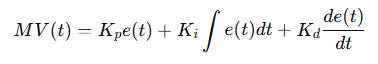
Where:
MV = Manipulated Variable (controller output)
e(t) = Error (SP − PV)
Kp = Proportional gain
Ki = Integral gain
Kd = Derivative gain
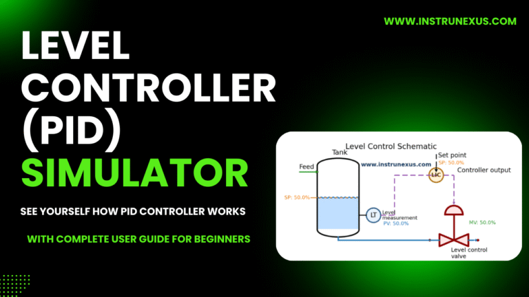
Click here to try PID simulator:PID LEVEL CONTROLLER SIMULATOR
Each term contributes differently to the control response.
Understanding the Three PID Components
1. Proportional Control (P)
The proportional term generates an output that is proportional to the current error.
Example
If the setpoint is 100°C and the measured temperature is 90°C, the error is 10°C. The controller output will increase proportionally based on the proportional gain (Kp).
Key Characteristics
Advantages:
Provides immediate corrective action
Improves response speed
Limitations:
Cannot eliminate steady-state offset
Too high gain causes oscillations
Practical Example
In a temperature control loop, if Kp is too low:
The system responds slowly.
If Kp is too high:
The temperature oscillates around the setpoint.
2. Integral Control (I)
The integral term accumulates past errors and gradually increases the controller output until the error becomes zero.
Integral control is essential for removing steady-state offset.
Example
Suppose a pressure controller stabilizes at 48 bar instead of 50 bar. The integral action slowly increases the output until the pressure reaches the setpoint.
Key Characteristics
Advantages:
Eliminates steady-state error
Improves accuracy
Limitations:
Too much integral causes oscillations
Can cause integral windup
Integral Windup
Integral windup occurs when the controller continues integrating error even when the actuator is already at its maximum or minimum limit.
Example:
Control valve fully open
Controller still increasing integral output
Modern DCS systems implement anti-windup protection to avoid this issue.
3. Derivative Control (D)
The derivative term predicts the future behavior of the error by calculating its rate of change.
Derivative action helps dampen oscillations and improve stability.
Key Characteristics
Advantages:
Reduces overshoot
Improves system stability
Limitations:
Sensitive to measurement noise
Often avoided in noisy signals such as flow measurements
Practical Use
Derivative action is particularly useful in:
Temperature control loops
Slow processes
Processes with large inertia
Typical PID Control Loop Structure
A typical industrial control loop consists of several components.
↓
PID Controller
↓
Control Valve / Actuator
↓
Process
↓
Sensor / Transmitter
↓
Process Variable (PV)
This continuous feedback loop ensures that the process variable stays close to the desired setpoint.
Why PID Tuning is Important
Poorly tuned PID loops are extremely common in industrial plants. Surveys suggest that 30–40% of control loops in plants operate with suboptimal tuning.
Common problems include:
Slow response
Continuous oscillations
Large overshoot
Poor disturbance rejection
Instability
These issues can result in:
Reduced product quality
Increased energy consumption
Equipment wear
Safety risks
Proper PID tuning improves:
Process stability
Product consistency
Energy efficiency
Equipment life
Key Performance Characteristics of a Good PID Loop
A well-tuned control loop should achieve:
Fast Response
The system should reach the setpoint quickly after a change.
Minimal Overshoot
The process variable should not exceed the setpoint excessively.
Stability
The loop should not oscillate continuously.
Disturbance Rejection
The controller should quickly reject disturbances such as:
Load changes
Feed variations
Pressure fluctuations
Common PID Tuning Methods
Several methods exist for tuning PID controllers.
1. Manual Tuning Method
Manual tuning is the most common method used by field engineers.
Procedure
Step 1: Set
Kd = 0
Step 2: Increase Kp gradually until oscillations appear.
Step 3: Reduce Kp slightly to stabilize the system.
Step 4: Increase Ki slowly to eliminate steady-state error.
Step 5: Add small Kd to reduce overshoot.
This method works well for most industrial loops.
2. Ziegler–Nichols Tuning Method
The Ziegler–Nichols method is a classic tuning technique developed in the 1940s.
Step 1
Set:
Kd = 0
Step 2
Increase Kp until sustained oscillations occur.
The gain at this point is called:
Ultimate Gain (Ku)
Step 3
Measure the oscillation period:
Ultimate Period (Pu)
Step 4
Calculate tuning parameters:
| Controller | Kp | Ti | Td |
|---|---|---|---|
| P | 0.5 Ku | – | – |
| PI | 0.45 Ku | Pu / 1.2 | – |
| PID | 0.6 Ku | Pu / 2 | Pu / 8 |
This method provides aggressive tuning and may require fine adjustment.
3. Cohen–Coon Method
The Cohen–Coon method is designed for processes with dead time.
It provides better results for processes such as:
Heat exchangers
Distillation columns
Furnaces
This method requires identifying:
Process gain
Dead time
Time constant
4. Auto-Tuning
Modern control systems provide auto-tuning features.
Auto-tuning works by:
Applying small disturbances
Measuring process response
Calculating optimal PID parameters
Many DCS platforms include built-in auto-tuning tools.
Practical PID Tuning Example
Consider a tank level control loop.
System Description
Level transmitter
Control valve on inlet line
Setpoint: 60%
Initial Tuning
Ki = 0
Kd = 0
The level rises slowly.
Increase Kp
Response becomes faster but oscillates.
Reduce Kp
Oscillation reduces.
Add Integral
Offset disappears.
Add Derivative
Overshoot decreases.
Final result:
Stable response
No oscillation
Accurate control
Common PID Tuning Problems
Oscillations
Cause:
High proportional gain
Excessive integral action
Solution:
Reduce Kp
Reduce Ki
Slow Response
Cause:
Low proportional gain
Solution:
Increase Kp
Overshoot
Cause:
High Kp
High Ki
Solution:
Add derivative
Reduce Ki
Noisy Control Output
Cause:
Excessive derivative action
Solution:
Reduce Kd
Add signal filtering
Practical PID Tuning Tips for Engineers
Always start with P-only control.
Tune slow loops first, such as temperature loops.
Avoid using derivative action in noisy measurements.
Ensure control valves are properly sized.
Verify transmitter calibration before tuning.
Check process dynamics before adjusting PID parameters.
Use trend data from DCS historian.
Document tuning parameters for future reference.
Real Industrial Example: Temperature Control Loop
Consider a furnace temperature control system.
Challenges
Long time constant
Significant dead time
Recommended tuning:
Moderate proportional gain
Strong integral action
Small derivative action
Example parameters:
Ki = 0.4
Kd = 0.6
This configuration helps reduce temperature overshoot while maintaining stability.
Advanced PID Features in Modern DCS
Modern control systems include advanced PID features such as:
Feedforward Control
Anticipates disturbances before they affect the process.
Cascade Control
Uses two control loops:
Primary loop
Secondary loop
Example:
Temperature control using a flow control inner loop.
Gain Scheduling
Adjusts PID parameters depending on operating conditions.
When PID Control Is Not Enough
Some processes require advanced control techniques.
Examples include:
Multivariable processes
Highly nonlinear systems
Large dead-time processes
Advanced techniques include:
Model Predictive Control (MPC)
Adaptive Control
Fuzzy Logic Control
However, PID control still remains the backbone of industrial automation.
Understanding Process Parameters in PID Simulation
Modern PID tuning tools and training simulators allow engineers to adjust not only the controller parameters (Kp, Ki, Kd) but also the process dynamics. In the PID simulator used in this tutorial, the following process parameters can be adjusted interactively:
Process Gain (K)
Time Constant (τ)
Simulation Time
These parameters represent the dynamic behavior of the physical process being controlled.
Understanding these parameters is essential for successful PID tuning.
Process Gain (K)
Process Gain represents how strongly the process responds to a change in the controller output.
It can be defined as:
K=Change in Process Variable / Change in Manipulated Variable
In simple terms, it tells us how sensitive the process is.
Example
Suppose a control valve opening changes from 40% to 50%, and the tank level increases from 60% to 70%.
Process gain:
K= (70−60) / (50−40) =1
This means the process variable changes 1 unit for every unit change in controller output.
High Process Gain
If the process gain is high:
Small controller outputs cause large process changes
The system may become unstable
PID tuning must use lower Kp
Example processes with high gain:
Flow control loops
Pressure control loops
Low Process Gain
If the process gain is low:
The process responds slowly
Larger controller output is required
Example processes:
Large tanks
Thermal systems
Effect on PID Tuning
| Process Gain | Controller Action |
|---|---|
| High Gain | Reduce Kp |
| Low Gain | Increase Kp |
Time Constant (τ)
The time constant (Tau) represents how fast a process responds to a change.
It is the time required for the process to reach 63.2% of its final value after a step change.
Mathematical Representation
For a first-order process:
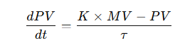
Where:
PV = Process Variable
MV = Manipulated Variable
K = Process Gain
τ = Time Constant
Practical Meaning
A small time constant means the process responds quickly.
Examples:
Flow control loops
Pressure loops
A large time constant means the process responds slowly.
Examples:
Furnace temperature control
Large tank level control
Example
Consider a tank level control system:
If the level eventually reaches 100%, the time constant is the time taken to reach:
63.2%63.2\%
of the final value.
Effect on PID Tuning
| Time Constant | Behavior |
|---|---|
| Small τ | Fast system |
| Large τ | Slow system |
Slow processes typically require:
Larger integral action
Moderate proportional gain
Simulation Time
Simulation time represents the total duration of the control system simulation.
In training simulators, this parameter allows engineers to observe how the system behaves over time.
Typical simulation durations include:
30 seconds → Fast processes
60 seconds → Medium processes
120 seconds or more → Slow thermal processes
Increasing simulation time helps engineers observe:
Oscillations
Settling behavior
Steady-state performance
How Process Dynamics Affect PID Tuning
The tuning parameters of a PID controller depend heavily on the process dynamics.
The main process characteristics include:
Process gain
Time constant
Dead time
Together, these parameters define how the process responds to controller actions.
Example Scenario
Consider a tank level control system with the following parameters:
Time Constant (τ) = 20 s
Simulation Time = 65 s
If the controller settings are:
Ki = 0.5
Kd = 0.1
The system may show:
Moderate response speed
Small overshoot
Stable behavior
If the process gain increases to:
The system may become unstable unless Kp is reduced.
Experimenting with the PID Simulator
Using the simulator, engineers can perform several experiments to understand control behavior.
Experiment 1 – Low Process Gain
τ = 20
Observation:
Slow response
Larger controller output required
Experiment 2 – High Process Gain
τ = 20
Observation:
Very sensitive system
Oscillation risk
Experiment 3 – Slow Process
τ = 40
Observation:
Very slow response
Requires stronger integral action
Experiment 4 – Fast Process
τ = 5
Observation:
Very quick response
Derivative action may improve stability
Why Process Modeling Is Important
Understanding process parameters such as gain and time constant allows engineers to develop a process model.
A process model is a mathematical representation of the plant behavior.
Process modeling is essential for:
PID tuning
Control system design
Dynamic simulation
Operator training simulators
Many modern engineering tools use first-order plus dead time (FOPDT) models for process identification.
Practical Tips for Engineers
When tuning PID loops in real industrial plants, engineers should always evaluate the process dynamics.
Important considerations include:
Measure the process gain through step testing.
Estimate the time constant from trend data.
Identify process dead time.
Tune the PID parameters accordingly.
Validate tuning through plant testing.
Conclusion
PID control remains one of the most powerful and widely used tools in industrial automation. Despite its simple mathematical formulation, proper tuning requires a solid understanding of process dynamics and controller behavior.
Instrumentation engineers play a critical role in ensuring control loops operate efficiently. By understanding the effects of proportional, integral, and derivative actions, engineers can optimize control loops for stability, responsiveness, and accuracy.
Whether using manual tuning, Ziegler–Nichols, or modern auto-tuning techniques, the ultimate goal remains the same: maintaining stable and efficient process operation.
A well-tuned PID loop not only improves plant performance but also enhances safety, energy efficiency, and product quality.