In the world of process control, the control valve plays a pivotal role. It is the final control element, the muscle that translates the brain’s (the controller’s) commands into physical action, meticulously regulating the flow of fluids to maintain process variables at their desired setpoints. However, the performance of this crucial component is not always as straightforward as we might hope. Three silent culprits – hysteresis, deadband, and response time – can stealthily sabotage the efficiency and stability of your entire control loop. For any engineer, technician, or student venturing into instrumentation and process control, a thorough understanding of these phenomena is not just beneficial; it’s essential for troubleshooting, optimization, and ensuring the smooth and safe operation of any plant.
This comprehensive guide will demystify control valve hysteresis, deadband, and response time. We will explore their definitions, delve into their underlying causes, analyze their detrimental effects on process control, and, most importantly, discuss practical strategies to measure, manage, and mitigate their impact.
The Ideal vs. The Real: A Quick Prelude
In a perfect world, a control valve would respond instantaneously and precisely to any change in the control signal. A 50% signal from the controller would result in the valve stem moving to exactly 50% of its travel, regardless of its previous position or the direction of the signal change. However, in the real world, mechanical and fluid dynamic imperfections introduce non-ideal behaviors. It is within this gap between the ideal and the real that we find hysteresis, deadband, and a finite response time.
Control Valve Hysteresis: The “Memory” Effect
What is Hysteresis?
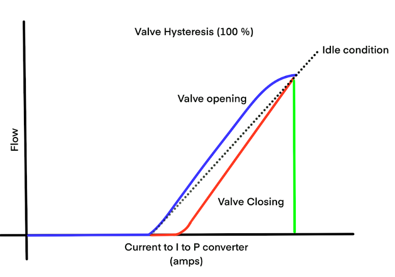
Imagine you’re trying to push a heavy box across a rough floor. You need a certain amount of force to get it moving. Once it’s in motion, you might find that it takes slightly less force to keep it moving in the same direction. Now, if you want to reverse the direction of the box, you’ll again need a significant push to overcome the static friction. This “lag” or difference in response based on the direction of applied force is analogous to hysteresis in a control valve.
In technical terms, control valve hysteresis is the phenomenon where the valve’s position for a given input signal depends on the direction of the signal change. For the same input signal value, the valve will be at a different position when it’s opening (upscale signal) compared to when it’s closing (downscale signal). This difference, typically expressed as a percentage of the valve’s full travel, creates a hysteresis loop when you plot the valve position against the input signal. A larger loop signifies more significant hysteresis.
What Causes Hysteresis?
The primary culprit behind control valve hysteresis is friction. This friction can manifest in several areas:
- Valve Packing Friction: The sealing system around the valve stem, known as the packing, is a major source of friction. Tighter packing, necessary to prevent leaks, increases this friction.
- Actuator Seal Friction: In pneumatic actuators, the seals on the piston or diaphragm contribute to the overall friction.
- Guide Bushing Friction: The bushings that guide the valve stem can also be a source of friction.
- Fluid Dynamic Forces: The pressure of the process fluid acting on the valve plug can create forces that oppose the actuator’s movement, contributing to a form of dynamic hysteresis.
- Mechanical Backlash: Loose linkages between the actuator and the valve stem can introduce play, which manifests as a form of hysteresis.
The Deleterious Effects of Hysteresis on Process Control
Hysteresis is a silent disruptor of process stability. Its presence can lead to:
- Limit Cycling: The controller, attempting to reach the setpoint, will constantly overshoot and undershoot, leading to a continuous oscillation around the desired value. This is because the controller’s output changes, but due to hysteresis, the valve doesn’t move until the change is large enough to overcome the friction. By the time the valve does move, the process variable has already deviated significantly, causing the controller to reverse its action, and the cycle repeats.
- Reduced Process Gain: The effective gain of the control loop is reduced, meaning the controller has to work harder to achieve the same change in the process variable.
- Increased Process Variability: The overall variability of the process increases, leading to inconsistent product quality and potential violations of operating limits.
- Slower Loop Response: The control loop becomes sluggish and less responsive to disturbances.
Measuring and Mitigating Hysteresis
Measuring hysteresis involves cycling the control valve through its full range of motion while recording the input signal and the actual stem position. The maximum difference between the upscale and downscale stem positions for the same input signal gives the hysteresis value.
To combat the effects of hysteresis, several strategies can be employed:
- Proper Valve Sizing and Selection: Selecting a valve with low-friction packing and a high-performance actuator is the first line of defense.
- Use of a Valve Positioner: A smart or digital valve positioner is a powerful tool to overcome hysteresis. The positioner has its own internal control loop that directly measures the stem position and adjusts the actuator pressure to ensure the valve reaches the desired position, regardless of friction. It essentially linearizes the valve’s response.
- Proper Maintenance: Regular lubrication of the valve stem and actuator, as well as periodic inspection and replacement of worn seals and packing, can significantly reduce friction.
- Advanced Control Strategies: In some cases, model-based control strategies can be used to compensate for the known hysteresis of a valve.
Understanding Deadband: The Zone of Inaction
What is Deadband?
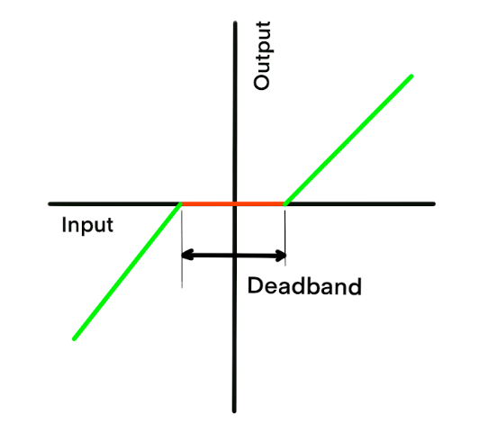
Imagine a car’s steering wheel with a bit of “play.” You can turn it a small amount in either direction before the wheels actually start to turn. This range of input where nothing happens is the deadband.
In a control valve, the deadband is the range of controller output signal change that fails to produce any movement of the valve stem. It is a zone of inaction. For instance, if a valve has a 1% deadband, a change in the controller output from 50% to 50.5% and back to 50% might not cause the valve to move at all. The signal must change by more than the deadband value to initiate a response.
What Causes Deadband?
Deadband in control valves is primarily caused by:
- Mechanical Backlash: This is the most common cause. Looseness in the linkages between the actuator stem and the valve stem, or worn-out gears in a geared actuator, creates a gap that must be taken up before any motion is transmitted to the valve.
- Actuator and Positioner In-sensitivity: A sluggish or poorly calibrated positioner can contribute to deadband.
- Friction (Stiction): While friction is the primary cause of hysteresis, a specific type of friction called “stiction” (static friction) can also contribute to deadband. Stiction is the force required to initiate movement from a resting position.
The Damaging Impact of Deadband on Process Control
Deadband is arguably more detrimental to process control than hysteresis. Its effects include:
- Limit Cycling: Similar to hysteresis, deadband is a major cause of limit cycling. The controller output changes, but the valve doesn’t respond. The process variable continues to drift away from the setpoint. The controller increases its output further until the deadband is overcome, at which point the valve moves, often overcorrecting the error. This leads to a sustained oscillation.
- Increased Process Variability: The presence of deadband directly translates to a less precise control and therefore, higher process variability.
- Poor Disturbance Rejection: The control loop’s ability to respond to and reject process disturbances is severely hampered.
Measuring and Mitigating Deadband
Deadband can be measured by making small, incremental changes to the controller output and observing the point at which the valve stem begins to move.
Strategies to minimize deadband include:
- High-Performance Actuators and Linkages: Using actuators with tight, backlash-free linkages is crucial.
- Digital Valve Positioners: Modern digital valve positioners are highly effective at eliminating the effects of deadband. They can make very small and precise adjustments to the actuator pressure to overcome any backlash and initiate valve movement with minimal change in the control signal.
- Proper Mechanical Assembly and Maintenance: Ensuring all mechanical connections are secure and free from excessive wear is a fundamental step in reducing deadband.
Hysteresis vs. Deadband: A Key Distinction
While both are non-linearities that degrade control performance, there’s a subtle but important difference:
- Hysteresis is a continuous, direction-dependent phenomenon. For any given input signal, there will be two different output positions.
- Deadband is a region of no response. The output remains fixed for a range of input signal changes.
In practice, many control valves exhibit a combination of both hysteresis and deadband.
Grasping Control Valve Response Time: The Need for Speed (and Precision)
What is Response Time?
Control valve response time refers to how quickly the valve can move to a new position after a change in the control signal. It’s a measure of the valve’s agility. A slow response time can be just as detrimental as hysteresis or deadband, especially in fast-acting processes.
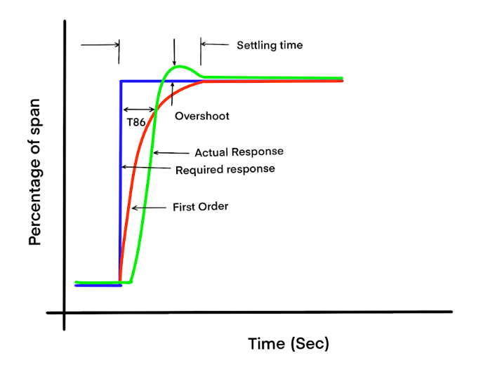
The response time of a control valve is often characterized by several parameters defined by ISA standards (like ISA-75.25.01), including:
- Dead Time (T0): The time delay between the initial change in the control signal and the first detectable movement of the valve stem.
- Time to 63.2% of Final Value (T63): The time it takes for the valve to reach 63.2% of its total travel in response to a step change in the input signal. This is a common metric used to characterize the speed of a first-order system.
- 86.5% Response Time (T86): The time taken to reach 86.5% of the final value.
- Overshoot: The amount by which the valve stem travels past its final intended position before settling.
Factors Influencing Response Time
Several factors determine how quickly a control valve can respond:
- Actuator Size and Type: Larger actuators generally require more air volume and will have a slower response time. The design of the actuator (e.g., spring-diaphragm vs. piston) also plays a role.
- Pneumatic Tubing Size and Length: The diameter and length of the tubing supplying air to the actuator significantly impact the response time. Longer, narrower tubing will result in a slower response.
- Air Supply Pressure: Higher air supply pressure can lead to a faster response, but it needs to be within the actuator’s design limits.
- Positioner Performance: The speed and tuning of the valve positioner are critical. A well-tuned digital positioner can significantly improve the response time.
- Valve and Trim Size: Larger, heavier plugs and stems will have more inertia and will naturally respond more slowly.
- Process Fluid Forces: High-pressure drops and fluid forces acting on the valve plug can oppose the actuator’s movement and slow down the response.
The Consequences of Poor Response Time
A slow control valve can lead to:
- Poor Disturbance Rejection: The valve cannot react quickly enough to counteract process disturbances, leading to larger deviations from the setpoint.
- Inability to Track Setpoint Changes: In processes where the setpoint changes frequently, a slow valve will lag behind, resulting in poor tracking performance.
- Process Instability: In very fast processes, a slow valve can introduce enough phase lag to destabilize the entire control loop.
Improving Control Valve Response Time
To enhance the responsiveness of a control valve, consider the following:
- Proper Actuator Sizing: The actuator should be sized to provide sufficient force and speed for the application.
- Use of a Volume Booster: For large actuators, a volume booster can be used to increase the rate of air flow to the actuator, thereby speeding up its response.
- Optimize Pneumatic Tubing: Use shorter lengths of larger diameter tubing to minimize pressure drop and volume delays.
- Tune the Positioner Aggressively (with caution): The tuning parameters of a digital positioner can often be adjusted to achieve a faster response. However, overly aggressive tuning can lead to overshoot and instability.
- Select the Right Valve for the Job: In high-speed applications, consider valve types that are inherently faster, such as rotary valves with smaller, lighter plugs.
Conclusion: A Call for Vigilance and Proactive Management
Hysteresis, deadband, and response time are not just abstract concepts for textbooks; they are real-world phenomena that have a tangible impact on the bottom line of any process industry. They can lead to wasted energy, off-spec product, increased equipment wear, and even safety hazards.
The key to mastering control valve performance lies in a proactive approach. It begins with the careful selection and sizing of valves and actuators. It continues with the judicious use of modern digital valve positioners, which are arguably the most effective tool in combating these non-linearities. And it is sustained through a diligent maintenance program that ensures the mechanical integrity of the final control element.
By understanding the causes and effects of hysteresis, deadband, and response time, and by implementing the strategies outlined in this guide, you can move from a reactive troubleshooting mode to a proactive optimization mindset. The result will be a more stable, efficient, and profitable process, all thanks to a deeper appreciation for the nuanced behavior of the humble yet critical control valve.